Opening requested calculation...

Please wait, this takes like 47 seconds. Thank you for your patience! :)

☠ 0 humans have been terminated by curable diseases since this page started loading

Listen Get

The Optimal Budget Generator: A Causal Inference Protocol for Maximizing Median Health and Wealth Through Public Goods Funding

Generating Integrated Public Budget Recommendations Using Diminishing Returns Modeling and Cost-Effectiveness Analysis

Author

Affiliation

Mike P. Sinn

Institute for Accelerated Medicine

Abstract

Budget processes respond to lobbying intensity and historical precedent rather than causal evidence of effectiveness.

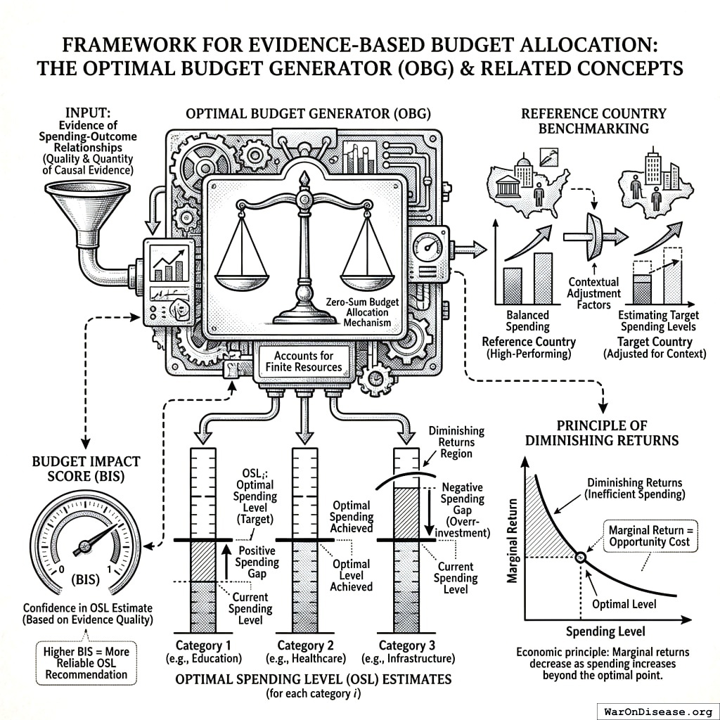
The Optimal Budget Generator (OBG) applies causal inference, diminishing returns modeling, cost-effectiveness analysis, and efficiency frontiers to choose the size and the composition of public spending that maximize two terminal general-welfare metrics: real after-tax median income growth and median healthy life years. The total budget is an output, not an input: every program must beat two outside options, a universal cash payment and leaving the money with taxpayers, so the model can recommend a smaller budget as well as a different one. For each goal, OBG compares delivery methods (public provision, vouchers, cash, prizes, payment for results) against cash and estimates an Optimal Spending Level (OSL) identifying where marginal returns equal those of the best alternative use.

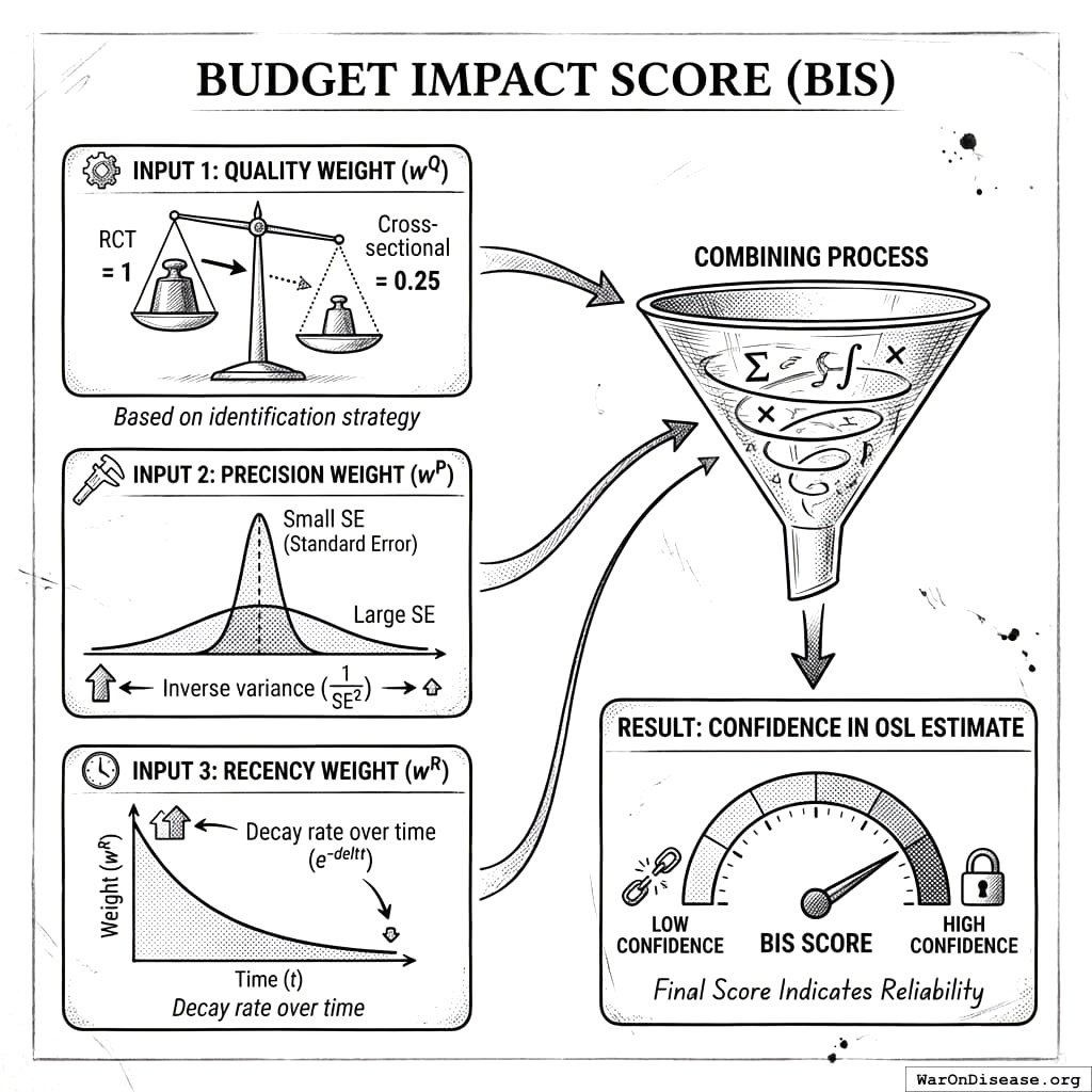
The Budget Impact Score (BIS) measures confidence in each OSL estimate based on study quality, statistical precision, and temporal recency of the underlying causal evidence. The result is a gap analysis showing which categories are over- or underfunded relative to evidence-based targets, enabling systematic reallocation from low-return to high-return public investments. At system scale, the model’s Optimal Governance Trajectory reaches 56.7x (90% CI: 21x-148x) the Earth baseline after 20 years, raises average income to $1.16 million (90% CI: $429,664-$3.04 million) versus $20,483 on the status-quo path, reaches $10.7 quadrillion (90% CI: $3.95 quadrillion-$28 quadrillion) in total output, and recovers roughly $101 trillion (90% CI: $59.6 trillion-$161 trillion)/year in suppressed value (The Political Dysfunction Tax).

Keywords

budget optimization, optimal budget generator, evidence-based policy, meta-analysis, cost-effectiveness, diminishing returns, cross-country analysis, public finance, welfare economics, spending targets

Abstract

Your government decides how much to spend on each category the same way it has for decades: last year’s number, plus whatever the loudest lobbyist got added, minus whatever the latest crisis forced a cut on. This is called “the budget process.” It has no optimization function. It has no feedback loop. It has no measurable objective. It is, in the technical sense, not a process at all. It is an accident that repeats annually.

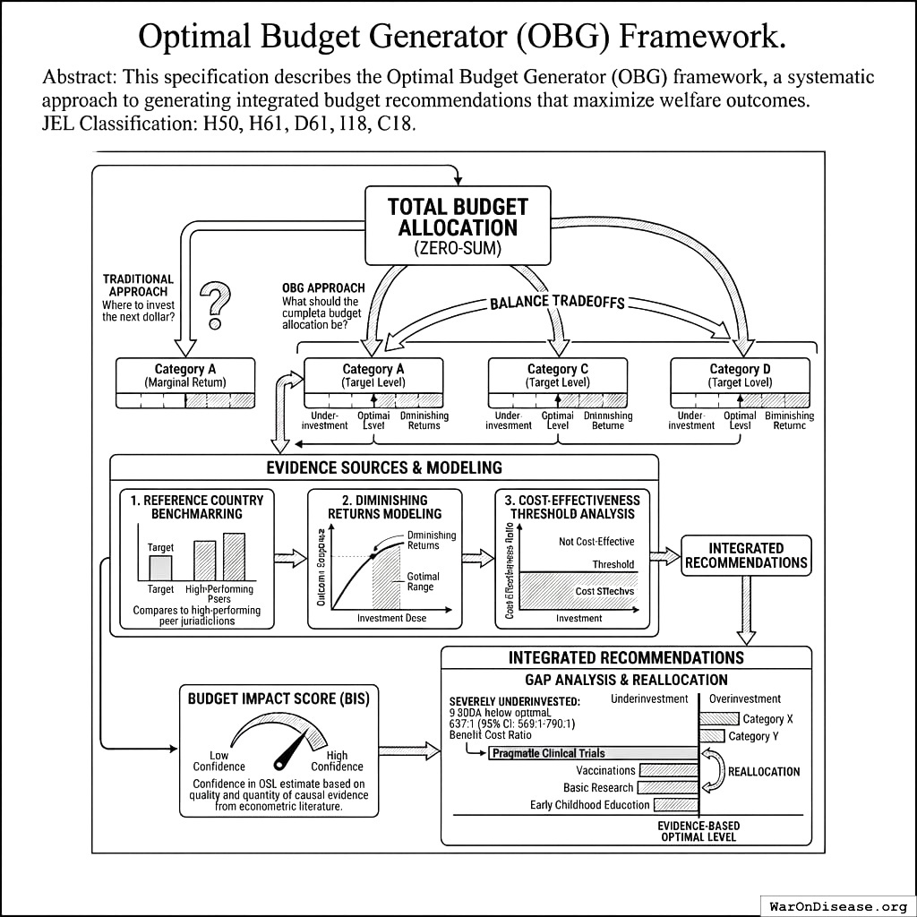
This specification describes the Optimal Budget Generator (OBG) framework, a systematic approach to generating integrated budget recommendations that maximize welfare as measured by two terminal general-welfare metrics: real after-tax median income growth and median healthy life years.

Three ways to figure out optimal spending combine to show the gap between what you spend and what you should spend. The gap is filled with lobbyists.

JEL Classification: H50, H61, D61, I18, C18

Unlike marginal-return frameworks that ask “where should we invest the next dollar?”, OBG asks “what should the complete budget allocation be?” Each category has a target level - too little means underinvestment, too much means diminishing returns. But unlike the Recommended Daily Allowance for nutrients (where you can meet all targets simultaneously), every budget dollar has other uses: another category, a universal cash payment, or staying with the taxpayer who earned it. OBG generates integrated recommendations that compare all of these uses, so the total budget is an output of the model, not an input.

The framework combines three evidence sources: (1) diminishing returns modeling from dose-response studies, (2) cost-effectiveness threshold analysis from health economics, and (3) efficiency frontiers, which separate waste from diminishing returns and, for defense, price the least-cost capabilities that defending the country requires. Neither peer-country spending nor current spending ever sets a target by itself. The Budget Impact Score (BIS) measures our confidence in each category’s OSL estimate based on the quality and quantity of causal evidence from the econometric literature.

The result is a gap analysis showing which categories are below evidence-based optimal levels, enabling systematic reallocation from overinvestment to underinvestment. Applied to the US federal budget, the illustrative example identifies pragmatic clinical trials as the most severely underinvested category (current spending is about 1% of the OSL, and the platform that runs these trials returns 439 (90% CI: 321-600):1 in R&D cost savings alone), followed by vaccinations, and identifies military spending as the largest overinvestment ($702 billion (90% CI: $671 billion-$728 billion) above the threat-based cost frontier). Basic research and early childhood education have strong evidence that more spending helps, but their OSLs are not derived yet.

Scale note. If budget allocation is the core bottleneck, the upside from fixing it is civilization-scale. Under the project’s best-case governance ceiling, the recoverable upside is $101 trillion (90% CI: $59.6 trillion-$161 trillion) per year. Over 20 years, the Optimal Governance Trajectory reaches 56.7x (90% CI: 21x-148x) the Earth baseline, raises average income to $1.16 million (90% CI: $429,664-$3.04 million) versus $20,483 on the status-quo path, and reaches $10.7 quadrillion (90% CI: $3.95 quadrillion-$28 quadrillion) in total output. This specification focuses on the allocation layer of that plan; the full derivation lives in The Political Dysfunction Tax¹.

System Overview

What Policymakers See

A dashboard showing spending gaps by category, with clear recommendations:

Illustrative Example: US Federal Budget Gap Analysis

The following table demonstrates how OBG output would appear.

Warning

Illustrative data. This table shows the output format, not a recommendation. Each OSL has a stated basis: a worked example in this paper (see Worked Example: Pragmatic Clinical Trials and Worked Example: Vaccinations), the threat-based cost frontier for the military (see Worked Example: Military Spending as a Cost Frontier), or the cash benchmark. Rows marked “Not derived” show only the direction of the evidence. OBG does not fill them with a multiple of current spending, because a target anchored on today’s budget inherits today’s errors.

Category	Current	OSL	Gap	Basis	Evidence	Income Effect	Health Effect	Action
Pragmatic clinical trials	$0.5B	$50B	+$49.5B	Worked example	A (RCTs)	++	+++	Scale 100x
Vaccinations	$8B	$16B	+$8B	Worked example	A (RCTs)	+	+++	Increase
Military	$886 billion	$184 billion (90% CI: $158 billion-$215 billion)	Cut $702 billion (90% CI: $671 billion-$728 billion)	Threat-based cost frontier	C (assumption-based costs)	−	−	Decrease
Agricultural subsidies	$25B	$0B	-$25B	Cash benchmark	C (assumption)	−	−	Eliminate
Basic research	$45B	Not derived	Not derived	Evidence on direction only	Not graded	++	++	Estimate OSL; evidence says increase
Early childhood (0-5)	$50B	Not derived	Not derived	Evidence on direction only	Not graded	+++	+	Estimate OSL; evidence says increase
Universal cash payment	$0	Not estimated	Not estimated	Not estimated		++	+	Estimate

Positive gaps indicate underinvestment; negative gaps indicate overinvestment. Income Effect: impact on real after-tax median income growth. Health Effect: impact on median healthy life years. Scale: +++ strong positive, ++ moderate positive, + weak positive, − negative. Evidence grades rate confidence in the OSL, not in the category’s effects: early childhood programs have strong randomized evidence that more spending helps, but no estimate yet of the spending level where returns fall to the opportunity cost, so they have no OSL and no grade.

The cuts in these rows are much larger than the increases. The OBG does not force the difference into any row. The full model assigns each dollar to its highest-value use: another category, a universal cash payment, or lower taxes. This example does not estimate those curves yet, so the difference stays unassigned.

What Budget Analysts See

• OSL estimates with confidence intervals and methodology notes
• Cross-country spending data showing spending-outcome relationships
• Diminishing returns curves identifying optimal spending levels
• Evidence quality scores (BIS) for each category
• Sensitivity analysis showing how OSL changes with different assumptions
• Priority rankings by gap size weighted by evidence confidence

Where This Fits

+-------------------------------------------------------------+
|                    OPTIMOCRACY FRAMEWORK                     |
+-------------------------------------------------------------+
|                                                              |
|  +---------------------+    +-----------------------------+  |
|  |  Budget Generator   |    |  Policy Generator           |  |
|  |  (OBG/BIS Framework)|    |  (OPG/PIS Framework)        |  |
|  |                     |    |                             |  |
|  |  Answers:           |    |  Answers:                   |  |
|  |  "How should we     |    |  "What policies should      |  |
|  |  allocate the       |    |  we adopt/change?"          |  |
|  |  budget?"           |    |                             |  |
|  |                     |    |                             |  |
|  |  Primary output:    |    |  Primary output:            |  |
|  |  Integrated budget  |    |  Enact/Replace/Repeal       |  |
|  |  recommendations    |    |  recommendations            |  |
|  +---------------------+    +-----------------------------+  |
|                                                              |
|  Both feed into: Constitutional Layer (outcome-optimizing rules)  |
+-------------------------------------------------------------+

The OBG/BIS framework answers: “Given what we know about returns to spending, what are the optimal allocation levels?”

Budget generator and policy generator both feed into constitutional rules. It’s checks and balances, but the checks can do maths.

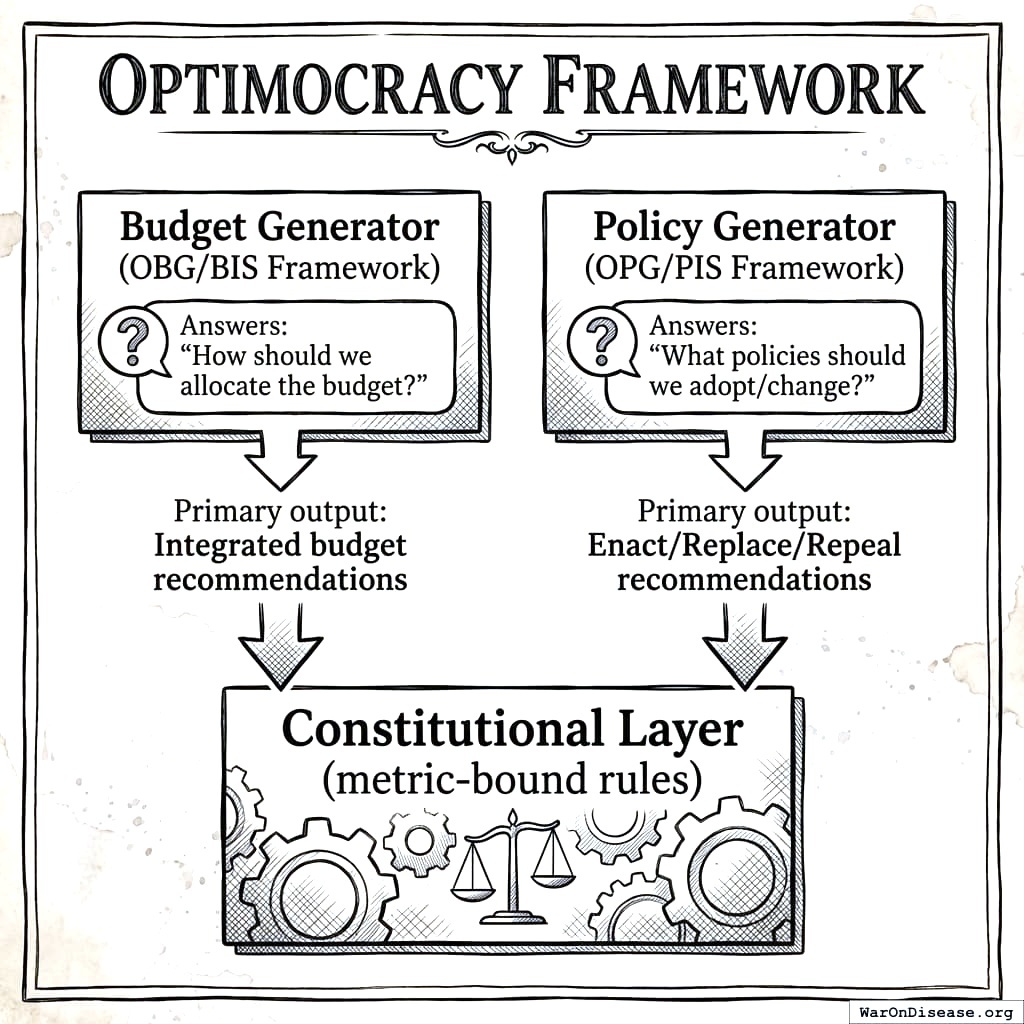
The OPG framework (see Optimal Policy Generator Specification²) answers: “Which policy reforms beyond budget allocation would most improve welfare?”

Implementation Mechanism

This specification focuses on generating evidence-based budget recommendations. Political implementation mechanisms are discussed separately in Incentive Alignment Bonds³.

Introduction

Why Budget Allocation Fails Today

Budget allocation is fundamentally a problem of social choice under uncertainty⁴. The challenge is not simply technical but institutional: current budget processes systematically diverge from welfare-optimal allocations because small, concentrated groups organize while large, diffuse ones do not⁵, because organized industries and pressure groups shape the rules and transfers written for them^6,7, and because even a planner with the right objective does worse deciding case by case than following a rule⁸.

Current budgets: lobbying and ‘we’ve always done it this way.’ Result: money goes to things that don’t work instead of things that do. Tradition is expensive.

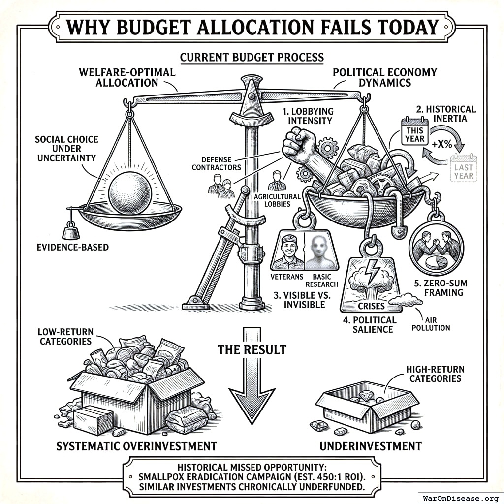
Current budget allocation follows a process dominated by:

1. Lobbying intensity: Categories with organized beneficiaries (weapons manufacturers, agricultural lobbies) receive disproportionate funding regardless of evidence
2. Historical inertia: This year’s budget is last year’s budget plus a percentage, not a fresh optimization
3. Visible vs. invisible beneficiaries: Programs with identifiable beneficiaries (veterans) outcompete programs with diffuse beneficiaries (clinical trials, vaccinations)
4. Political salience: Crises drive spending regardless of cost-effectiveness (terrorism vs. air pollution)
5. Zero-sum framing: Budget debates treat all categories as competing rather than asking which ones are at optimal levels

The result: systematic overinvestment in low-return categories and underinvestment in high-return categories. Historical examples demonstrate the scale of missed opportunities: the smallpox eradication campaign returned an estimated 159:1⁹, yet similar high-return public health investments remain chronically underfunded.

The RDA Analogy: Optimal Levels, Not Just Marginal Returns

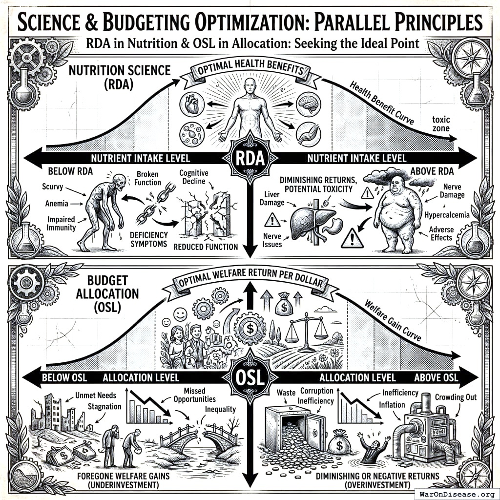
Nutrition science doesn’t just say “eat more vitamins.” It specifies Recommended Daily Allowances - target intake levels where:

• Below RDA: Deficiency symptoms, reduced function
• At RDA: Optimal health benefits
• Above RDA: Diminishing returns, potential toxicity

Budget allocation should work the same way. For each spending category:

• Below OSL: Foregone welfare gains (underinvestment)
• At OSL: Optimal welfare return per dollar
• Above OSL: Diminishing or negative returns (overinvestment)

infinite spending on any category doesn’t make sense, even one with high returns. Early childhood education has excellent returns - but spending $10 trillion on it wouldn’t produce 10x the benefits of spending $1 trillion. There’s an optimal level.

Nutritionists tell you how much vitamin C you need. OSL tells governments how much education funding they need. One prevents scurvy, the other prevents stupid.

What This Framework Provides

Five pieces: evidence-based targets, gap analysis, priority ranking, uncertainty assessment, and wishful thinking. Wait, scratch that last one.

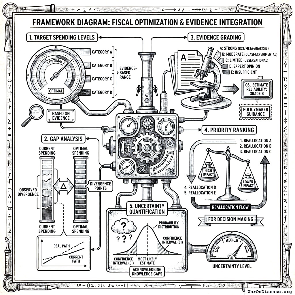
1. Target spending levels for each budget category based on evidence
2. Gap analysis showing where current spending diverges from optimal
3. Evidence grading so policymakers know which OSL estimates are reliable
4. Priority ranking for reallocation decisions
5. Uncertainty quantification around each estimate

Guarding Against Status-Quo Bias

A budget optimizer that starts from today’s budget can inherit today’s mistakes. Five design rules prevent this:

1. The total budget is a choice. The model does not hold total spending fixed. Every program must beat a universal cash payment and must beat leaving the money with taxpayers, after the cost of raising taxes. If no program beats them, the optimal budget is smaller.
2. Categories are goals, not agencies. A category is an outcome to buy (for example, child health), not an existing department. Each goal compares delivery methods: public provision, vouchers, cash, prizes and advance purchase commitments, payment for results, and rule changes that cost nothing.
3. Cash is the benchmark. A delivery method gets money only if it produces more welfare per dollar than giving the same dollar to people as cash.
4. Neither peer spending nor current spending is a target. If every government overspends on something, copying peers copies the error, and a target set as a multiple of today’s budget copies today’s error. Reference-country spending enters the efficiency frontier and dose-response models as data points. A category without a derived OSL shows “Not derived” and becomes a candidate for value-of-information pilots. An OSL from a frontier or from assumption-based costs, without causal evidence on returns, has a BIS of at most 0.59 (grade C, “pilot before scaling”).
5. New methods get pilots, not penalties. Most evaluations study programs that already exist, so a new delivery method has little evidence. Low evidence sends a method to pilot funding, not to exclusion.

Outcome Metrics: What We’re Optimizing

All OBG recommendations ultimately aim to maximize two terminal general-welfare metrics:

1. Real after-tax median income growth (pp/year): Year-over-year percentage change in inflation-adjusted, post-tax median household income. Sources: Census Bureau, BLS.

2. Median healthy life years (years): Expected years of life in good health at the population median. Sources: WHO Global Health Observatory, national health surveys.

The welfare function combines these with equal weight by default. The two metrics have different units (percentage points per year and years), so each is first divided by its cross-jurisdictional standard deviation, as in the OPG standardization:

\[ W = 0.5 \cdot \frac{\text{IncomeGrowth}}{\sigma_{\text{income}}} + 0.5 \cdot \frac{\text{HealthyYears}}{\sigma_{\text{health}}} \]

Why these two metrics? They are the terminal general-welfare metrics: the best currently measurable civilization-scale endpoints for approximating the terminal values defined in What Matters, pleasant consciousness and unpleasant consciousness. Most policy effects eventually show up in one or both. Economic policies (taxes, regulations, trade) primarily affect income growth. Health policies (healthcare access, public health, safety) primarily affect healthy life years. Education and infrastructure affect both. See Two-Metric Welfare Function for the complete framework.

Every spending category’s OSL is ultimately justified by its expected impact on these two metrics. The gap analysis and priority rankings reflect which reallocations would most improve the combined welfare function.

Related Work

The OBG framework builds on and extends several established traditions in public finance and evidence-based policy.

Budget Analysis Frameworks

Congressional Budget Office (CBO) Scoring. The CBO provides cost estimates for proposed legislation, projecting fiscal impacts over 10-year windows for bills that affect mandatory spending or revenues (5 years for bills that authorize discretionary programs)¹⁰. However, CBO scoring focuses on cost rather than welfare optimization - it answers “what will this cost?” not “what should we spend?” OBG complements CBO analysis by providing evidence-based spending targets against which proposals can be evaluated.

CBO scores costs. Performance budgeting measures results. Zero-based budgeting questions everything. OBG does all three and shows you the receipts.

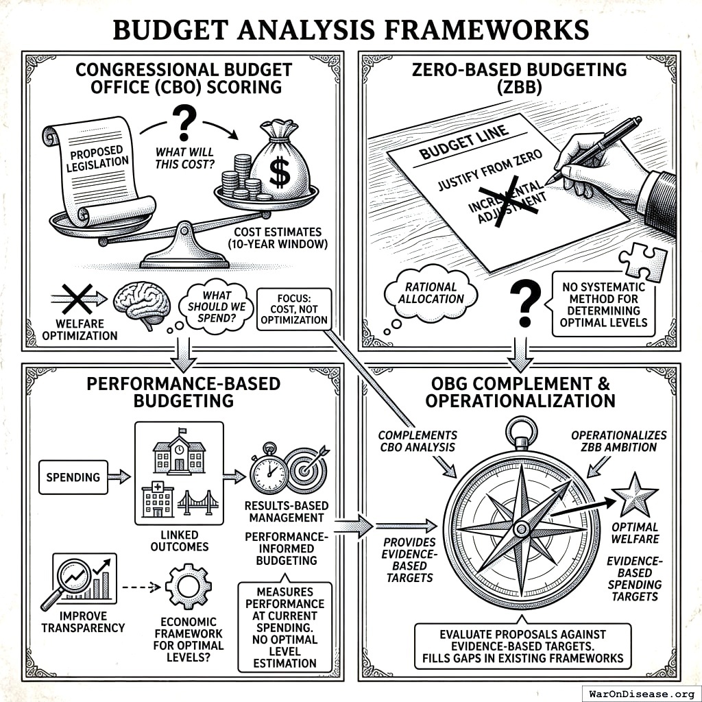
Performance-Based Budgeting. Since the Planning-Programming-Budgeting System (PPBS) of the 1960s, governments have attempted to link spending to outcomes. Modern variants include Results-Based Management and Performance-Informed Budgeting. These approaches improve transparency but typically lack the economic framework for determining optimal levels - they measure performance at current spending without estimating what spending should be.

Zero-Based Budgeting. ZBB requires justifying each budget line from zero rather than incremental adjustment. While philosophically aligned with OBG’s goal of rational allocation, ZBB provides no systematic method for determining optimal levels. OBG operationalizes ZBB’s ambition with evidence-based targets.

Evidence-Based Policy Movement

What Works Clearinghouses. Organizations like the What Works Clearinghouse (education), Cochrane Collaboration (health), and Campbell Collaboration (social policy) synthesize intervention evidence through systematic reviews. OBG draws on these evidence bases but extends beyond intervention evaluation to budget-level optimization. While clearinghouses answer “does this work?”, OBG answers “how much should we spend?”

Old way: evaluate programs one at a time. New way: optimize entire budgets at once. It’s like organizing your whole kitchen instead of just the spoon drawer.

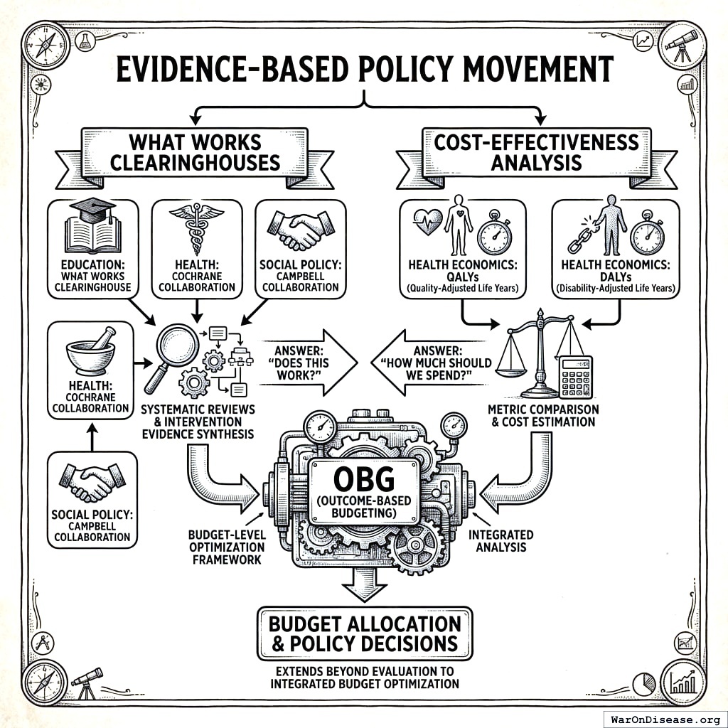
Cost-Effectiveness Analysis. Health economics has developed methods for comparing interventions using metrics like QALYs (Quality-Adjusted Life Years) and DALYs (Disability-Adjusted Life Years)¹¹. OBG incorporates cost-effectiveness as one of three estimation methods but applies it within an integrated budget optimization framework rather than intervention-by-intervention.

Comparative Public Finance

OECD Government Spending Analysis. The OECD publishes extensive cross-country spending comparisons and outcome data^12,13. OBG leverages this data infrastructure for diminishing returns analysis while adding the conceptual framework of optimal levels and evidence-weighted confidence.

A conceptual model showing the methodological progression from standard OECD benchmarking to OBG’s causal identification framework and actionable spending targets.

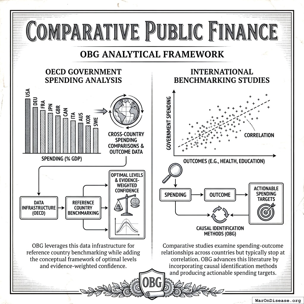
International Benchmarking Studies. Comparative studies examine spending-outcome relationships across countries but typically stop at correlation. OBG advances this literature by incorporating causal identification methods and producing actionable spending targets.

Budget-Allocation Models and Priority-Setting Systems

Policy Priority Inference. This computational model links how a government spreads its budget across programs to the expected movement of development indicators¹⁴. A UNDP study of Colombia projected that only 18% of Sustainable Development Goal indicators would reach their 2030 targets at the current pace, and that a 20% budget increase would raise this only to 20%; the authors report that reallocation would do more than adding money¹⁵. This supports OBG’s focus on diminishing returns. Unlike OBG, the model targets fixed indicator goals rather than a welfare function, and it calibrates on one country’s history rather than on causal estimates across jurisdictions.

Optima. Optima computes the split of a fixed HIV budget across programs that best meets goals such as fewer infections¹⁶. For 44 countries, optimal allocation of existing HIV budgets over 2016 to 2030 could avert about 7.4 million additional infections, a 26% drop in incidence, with no new money¹⁷. Sudan and Belarus moved their actual HIV budgets toward the recommended allocation¹⁸. Optima is the strongest evidence that budget optimization can change real budgets, within one sector.

Priority-setting systems. Disease Control Priorities^19,20, the Lancet Commission on Investing in Health²¹, the WHO “best buys”²², the Copenhagen Consensus²³, and the Washington State Institute for Public Policy²⁴ publish ranked lists of high-return spending. OBG uses these rankings as inputs to its cost-effectiveness method. Their common limit is adoption, which OBG leaves to the Incentive Alignment Bonds mechanism.

Evidence on budget size and composition. In rich countries, a government larger by 10 percentage points of GDP is associated with 0.5 to 1 percentage point lower annual growth, a correlation the authors warn against reading as causal²⁵. Public investment and education raise long-run growth, while pensions and subsidies lower it²⁶. About 30% of the potential gains from public investment are lost to inefficiency²⁷. Optimal research and development spending is at least two to four times actual US spending²⁸, and the optimal health share of spending rises with income²⁹. These results set the direction for categories whose OSLs are not derived yet. They do not set levels.

Efficiency frontiers. Frontier methods estimate the most output that any producer gets from a given input. Data envelopment analysis estimates the frontier from observed inputs and outputs, with weights taken from the data³⁰, and stochastic frontier analysis splits the error into symmetric random noise and a one-sided inefficiency term³¹. Applied to public spending, these methods measure how far each government is from best practice³². OBG uses the frontier’s slope as the best attainable marginal return (see Efficiency Frontier Analysis).

For a full survey, see Related Work in the Optimocracy paper³³.

How OBG Differs

The OBG framework advances existing approaches in four key ways:

1. Integrated multi-method estimation. Rather than relying on a single approach, OBG combines OSL estimates from diminishing returns modeling, cost-effectiveness analysis, and efficiency frontiers, and it never uses peer or current spending as a target. This provides robustness and identifies where methods agree or conflict.

Three different ways to count money, then deciding where to put it, then measuring how confident you are that you counted correctly. Like checking your restaurant bill three times because you still don’t trust yourself.

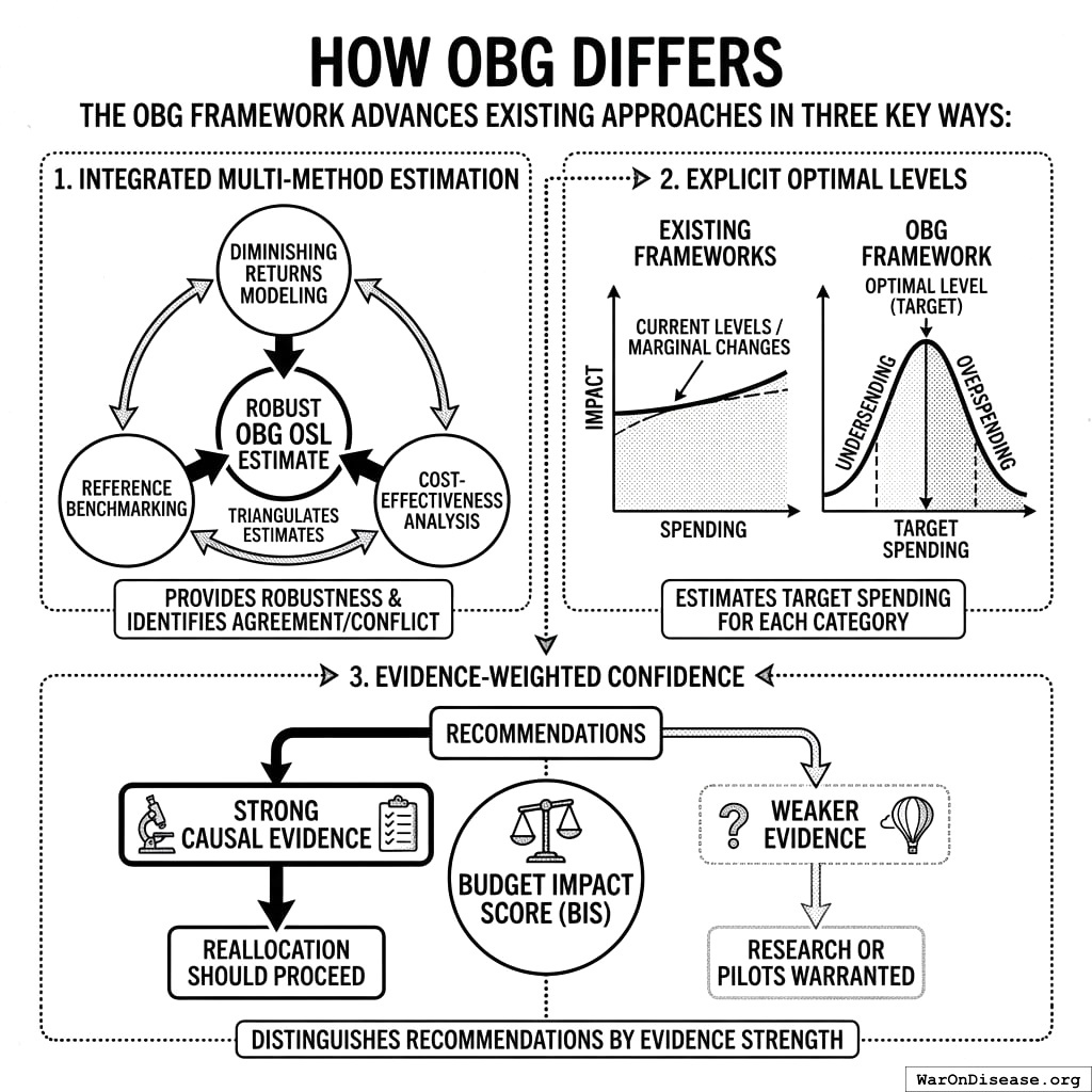
2. Explicit optimal levels. Unlike frameworks that analyze spending at current levels or propose marginal changes, OBG estimates target spending levels for each category - acknowledging that both underspending and overspending are suboptimal.

3. Evidence-weighted confidence. The Budget Impact Score (BIS) distinguishes recommendations supported by strong causal evidence (where reallocation should proceed) from those based on weaker evidence (where research or pilots are warranted).

4. Size and delivery are choices. Most budget tools take the total budget and the existing programs as given. OBG lets the total shrink when no program beats a universal cash payment or lower taxes, and it compares delivery methods for each goal against cash (see Delivery Methods and the Cash Benchmark).

Theoretical Framework

This section formalizes the OBG framework as a social planner’s optimization problem, establishing the theoretical foundations for optimal spending levels and evidence-weighted allocation.

A social planner is someone who plans society. They take evidence, weigh it (not literally), and decide how much money to spend on things. It’s like meal planning but for countries.

The Social Planner’s Problem

Consider a social planner who chooses both the total budget \(B\) and its allocation. Welfare is measured using the two-metric framework: real after-tax median income growth and median healthy life years.

Why these specific metrics? They are universal instrumental goods: virtually everyone wants higher purchasing power and longer healthy life, regardless of other values. They are hard to game (improving them requires actually helping typical citizens), measured by independent statistical agencies, and capture most policy effects. GDP can rise while median income stagnates; this framework correctly identifies such outcomes as low-welfare.

There are \(n\) goals (for example child health, basic research, or defense). Each goal \(i\) can be pursued through delivery mechanisms \(m \in \mathcal{M}_i\): direct public provision, vouchers, earmarked cash, prizes or advance purchase commitments, payment for results, or a rule change with no budget cost. Two outside options compete with every goal:

• a universal cash payment \(c\) (for example, a universal basic income), with spending \(s_c\); and
• lower taxes: revenue that is never raised, so the money stays with the people who earned it.

Let \(s_{im}\) denote spending on goal \(i\) through mechanism \(m\), so that \(B = \sum_{i}\sum_{m} s_{im} + s_c\). Mechanisms for the same goal are substitutes: public vaccination and vaccination vouchers reach the same unvaccinated people. To avoid counting the same high-return opportunities twice, welfare is defined per goal, not per mechanism. Each mechanism produces output toward its goal (for example, people vaccinated), \(q_{im} = f_{im}(s_{im})\), and the goal’s welfare depends on its total output \(q_i = \sum_{m} q_{im}\). If two mechanisms reach different populations, they serve different goals and are modeled as separate goals.

Each goal’s total output produces effects on both welfare metrics:

• \(\beta_{i}^{inc}(q_{i})\): Effect on real after-tax median income growth (pp/year)
• \(\beta_{i}^{hlth}(q_{i})\): Effect on median healthy life years (years)

Welfare from goal \(i\) follows the two-metric welfare function, with each metric divided by its cross-jurisdictional standard deviation so that the units match:

\[ W_{i}(q_{i}) = \alpha \cdot \frac{\beta_{i}^{inc}(q_{i})}{\sigma_{\text{income}}} + (1-\alpha) \cdot \frac{\beta_{i}^{hlth}(q_{i})}{\sigma_{\text{health}}} \]

where \(\alpha = 0.5\) by default (equal weight to economic and health welfare). \(W_c(s_c)\) is defined the same way for the universal cash payment. All welfare calculations in this framework flow through these two metrics.

Raising revenue has a welfare cost. A dollar of tax costs taxpayers more than a dollar, because taxes distort work, saving, and investment. Let \(C(B)\) be the welfare cost of raising \(B\) in taxes, measured in the same standardized units. Its derivative \(C'(B)\) is the marginal cost of public funds converted to welfare units³⁴.

Assumption 1 (Diminishing Returns). Each production function \(f_{im}\), each goal’s effect functions, and the cash payment’s effect functions are twice continuously differentiable, increasing, and concave. \(C(B)\) is increasing and convex.

The social planner maximizes aggregate welfare net of the cost of raising revenue:

\[ \max_{B,\,\{s_{im}\},\,s_c} \; \sum_{i=1}^{n} W_{i}\Big(\sum_{m \in \mathcal{M}_i} f_{im}(s_{im})\Big) + W_c(s_c) - C(B) \quad \text{subject to} \quad \sum_{i}\sum_{m} s_{im} + s_c = B, \quad s \geq 0 \]

Proposition 1 (Equimarginal Principle with Outside Options). At the optimum, every funded use of money has the same marginal welfare, and that common value equals the marginal cost of raising revenue:

\[ \begin{gathered} W_{i}'(q_{i}^*)\, f_{im}'(s_{im}^*) = W_c'(s_c^*) = C'(B^*) = \lambda^* \\ \text{for every funded mechanism, and for the cash payment if } s_c^* > 0 \end{gathered} \]

A mechanism with \(W_{i}'(q_i^*)\, f_{im}'(0) < \lambda^*\) receives no money. Because the goal’s welfare depends only on total output, a second mechanism that reaches the same people adds no welfare beyond the output it produces, so duplicate mechanisms cannot raise the optimal budget.

Proof. The Lagrangian is \(\mathcal{L} = \sum_{i} W_{i}\big(\sum_m f_{im}(s_{im})\big) + W_c(s_c) - C(B) - \lambda\left(\sum_{i,m} s_{im} + s_c - B\right)\). The first-order condition for \(B\) gives \(C'(B^*) = \lambda^*\). The first-order condition for each \(s_{im}\) gives \(W_i'(q_i^*) f_{im}'(s_{im}^*) = \lambda^*\) at interior solutions and \(W_i'(q_i^*) f_{im}'(0) \leq \lambda^*\) at corner solutions; the condition for \(s_c\) is analogous. Concavity of each \(W_i \circ \sum_m f_{im}\) and of \(W_c\), and convexity of \(C\), make these conditions sufficient. \(\square\)

Proposition 1 has three practical consequences:

1. Cash benchmark. Where the cash payment is funded, a delivery mechanism gets money only if its marginal welfare per dollar exceeds that of cash.
2. The total budget is an output. If no use of money beats the marginal cost of raising it, the optimal budget is smaller than the current one.
3. No forced spending of savings. Money cut from an over-funded category does not have to go to any particular category. It goes to the highest-value use, which can be another goal, the cash payment, or lower taxes.

Goals whose value depends on rivals. For most goals, welfare depends only on the country’s own output: a vaccinated child is protected whatever another country spends on vaccines. Defense is different, because many of the means by which a state tries to increase its security decrease the security of others³⁵. Welfare from defense therefore depends on rival spending \(s_{-d}\), and rival spending raises the marginal value of a country’s own defense:

\[ W_d = W_d(q_d;\, s_{-d}), \qquad \frac{\partial W_d}{\partial s_{-d}} < 0, \qquad \frac{\partial^2 W_d}{\partial q_d\, \partial s_{-d}} > 0 \]

A national planner takes \(s_{-d}\) as given, so Proposition 1 gives that country’s best response, and every country’s best response rises with the others’ spending. If all countries cut together, each country’s marginal value of defense falls, each defense OSL falls, and the freed money moves to its next-best use. No single planner can make that move, because it needs the others to move too. This is the reason the 1% Treaty^{36 37} cuts military spending by agreement instead of by one country. The treaty sends its money to clinical trials, which is consistent with consequence 3 while the treaty’s flow ($27.2 billion per year worldwide) stays below the trial gap (+$49.5B for the United States alone in the worked example).

Optimal Spending Levels Under Uncertainty

In practice, the welfare functions \(W_i(\cdot)\) are not known with certainty. Let \(\hat{W}_i(s)\) denote the planner’s estimate of welfare, with associated uncertainty \(\sigma_i^2(s)\).

Definition 1 (Optimal Spending Level). The Optimal Spending Level for category \(i\) is:

\[ \text{OSL}_i \equiv \arg\max_{s_i} \mathbb{E}[\hat{W}_i(s_i)] - \frac{\rho}{2} \text{Var}[\hat{W}_i(s_i)] \]

where \(\rho \geq 0\) is the planner’s risk aversion parameter.

For risk-neutral planners (\(\rho = 0\)), OSL reduces to the spending level that maximizes expected welfare. For risk-averse planners, OSL accounts for estimation uncertainty.

OBG does not build a mean-variance portfolio frontier across categories. When the risks of a public investment are borne by the public, the total cost of bearing them is insignificant, so the government should ignore uncertainty when it evaluates public investments³⁸. The result assumes that a program’s returns are independent of national income. The default is therefore \(\rho = 0\), and uncertainty enters through value of information: uncertain categories get pilots that reduce the uncertainty. A positive \(\rho\) is reserved for risks that spreading does not remove, such as an error in an assumption that many categories share.

Proposition 2 (OSL Characterization). Under Assumption 1, with estimated marginal welfare \(\hat{W}_i'(s)\) and estimation variance \(\sigma_i^2(s)\), the OSL satisfies:

\[ \mathbb{E}[\hat{W}_i'(\text{OSL}_i)] = r + \rho \cdot \frac{\partial \sigma_i^2}{\partial s}\bigg|_{s=\text{OSL}_i} \]

where \(r\) is the opportunity cost of public funds: the marginal welfare \(\lambda^*\) of the best alternative use of the last dollar (another goal, the universal cash payment, or lower taxes).

Proof. The first-order condition for the uncertainty-adjusted maximization problem yields the result. The term \(r\) represents the marginal value of funds in their best alternative use; the second term adjusts for risk. \(\square\)

Budget Impact Score as Precision Weighting

The Budget Impact Score formalizes the precision of OSL estimates, enabling evidence-weighted reallocation decisions.

Definition 2 (Budget Impact Score). For category \(i\) with \(n_i\) effect estimates \(\{\hat{\beta}_{ij}\}_{j=1}^{n_i}\), the Budget Impact Score is:

\[ \text{BIS}_i = \min\left(1, \frac{1}{K} \sum_{j=1}^{n_i} w_j^Q \cdot w_j^P \cdot w_j^R \right) \]

where:

• \(w_j^Q \in (0,1]\) = quality weight based on identification strategy (RCT = 1, cross-sectional = 0.25)
• \(w_j^P = 1/\text{SE}(\hat{\beta}_j)^2\) = precision weight (inverse variance)
• \(w_j^R = e^{-\delta(t_{now} - t_j)}\) = recency weight with decay rate \(\delta\)
• \(K\) = calibration constant

Proposition 3 (BIS as Inverse Variance). Under standard meta-analytic assumptions, BIS is proportional to the precision of the pooled effect estimate:

\[ \text{BIS}_i \propto \frac{1}{\text{Var}(\hat{\beta}_i^{pooled})} \]

where \(\hat{\beta}_i^{pooled}\) is the quality-weighted pooled estimate of spending effects.

Three ingredients that tell you how much to trust a number: how good it is, how exact it is, and how old it is. Like checking the expiration date on milk, but for statistics.

Gap Analysis and Welfare Gains

Definition 3 (Spending Gap). The spending gap for category \(i\) is:

\[ \text{Gap}_i = \text{OSL}_i - s_i^{current} \]

Proposition 4 (Welfare Gains from Gap Closure). For small gaps, the welfare gain from moving spending from current level to OSL is approximately:

\[ \Delta W_i \approx W_i'(s_i^{current}) \cdot \text{Gap}_i - \frac{1}{2} |W_i''(\bar{s})| \cdot \text{Gap}_i^2 \]

where \(\bar{s}\) is between \(s_i^{current}\) and \(\text{OSL}_i\).

Proof. Taylor expansion of \(W_i(\text{OSL}_i) - W_i(s_i^{current})\) around \(s_i^{current}\). \(\square\)

Corollary 1 (Priority Ranking). Categories should be prioritized for reallocation in order of:

\[ \text{Priority}_i = |\text{Gap}_i| \times \text{BIS}_i \times |W_i'(s_i^{current})| \]

This ranks categories by expected welfare gain adjusted for estimation confidence.

Note: In the simplified implementation used in the priority ranking example, we normalize by setting \(|W_i'(s_i^{current})| = 1\) for all categories, reducing the priority formula to \(\text{Priority}_i = |\text{Gap}_i| \times \text{BIS}_i\). This assumes equal marginal welfare weights across categories as a first approximation. Future iterations could incorporate category-specific marginal welfare estimates.

Welfare Bounds Under Model Uncertainty

When the functional form of \(W_i(\cdot)\) is uncertain, we can establish bounds on welfare gains.

Proposition 5 (Welfare Bounds). Let \(\underline{W}_i\) and \(\overline{W}_i\) denote lower and upper bounds on the welfare function consistent with available evidence. Then:

\[ \underline{\Delta W} = \sum_{i: \text{Gap}_i > 0} \underline{W}_i'(s_i) \cdot \text{Gap}_i \leq \Delta W \leq \sum_{i: \text{Gap}_i > 0} \overline{W}_i'(s_i) \cdot \text{Gap}_i = \overline{\Delta W} \]

The OBG framework reports both point estimates and these bounds via sensitivity analysis.

Summary of Theoretical Results

Result	Implication for OBG
Proposition 1	Optimal allocation equalizes marginal returns across goals, the cash payment, and the cost of raising revenue
Proposition 2	OSL accounts for both expected returns and uncertainty
Proposition 3	BIS captures estimation precision
Proposition 4	Gap closure yields quantifiable welfare gains
Corollary 1	Priority ranking optimizes reallocation sequence
Proposition 5	Welfare bounds enable robust recommendations

Core Methodology

Spending Category Data Structure

Boxes connected by lines. The boxes represent different kinds of information. The lines mean they’re related. It’s a family tree for spreadsheets.

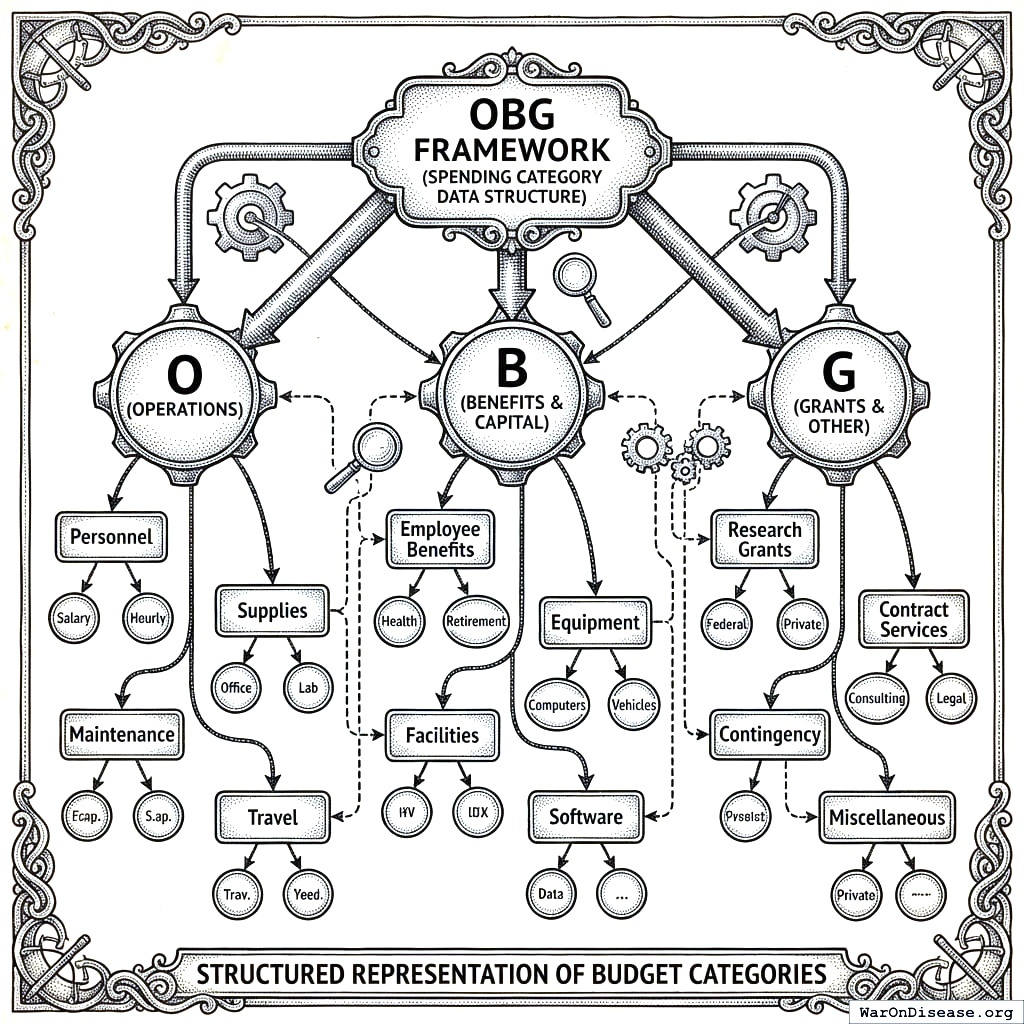
The OBG framework uses a structured representation of budget categories:

-- Spending categories
spending_categories (
    id, name, parent_category_id,
    spending_type, -- 'program', 'transfer', 'investment', 'regulatory'
    outcome_categories, -- which welfare outcomes this affects
    current_spending_usd, fiscal_year,
    data_source, last_updated
)

-- Cross-country spending data
reference_spending (
    category_id, country_code, year,
    spending_usd, spending_per_capita,
    spending_pct_gdp, population, gdp,
    data_source
)

-- Optimal spending level estimates (one row per goal and delivery mechanism)
osl_estimates (
    category_id, delivery_mechanism, -- 'public_provision', 'voucher', 'cash', 'prize', 'payment_for_results', 'rule_change'
    estimation_method, -- 'diminishing_returns', 'cost_effectiveness', 'efficiency_frontier', 'cost_frontier'
    osl_usd, osl_per_capita, osl_pct_gdp,
    confidence_interval_low, confidence_interval_high,
    evidence_grade, bis_score,
    methodology_notes, last_updated
)

-- Outside options that every use of money must beat
outside_options (
    option, -- 'universal_cash_payment', 'lower_taxes'
    marginal_welfare_per_dollar, confidence_interval_low, confidence_interval_high,
    data_source, last_updated
)

-- Gap analysis
spending_gaps (
    category_id, current_spending_usd,
    osl_usd, gap_usd, gap_pct,
    priority_score, -- gap * BIS confidence
    recommended_action
)

Three Methods for OSL Estimation

Method	Use Case	Data Required	Strengths	Limitations
Diminishing returns modeling	Categories with spending-outcome data across jurisdictions	Effect estimates at multiple spending levels	Theoretically grounded, finds optimal “knee”	Requires sufficient variation in spending
Cost-effectiveness threshold	Health/life-saving interventions	Cost per QALY/DALY, willingness-to-pay	Links to standard health economics11,39	Limited to monetizable outcomes
Efficiency frontier	Categories with measurable outputs across jurisdictions; for defense, a cost frontier built from the cost of each needed capability	Spending and outcomes in many jurisdictions, or capability costs	Separates waste from diminishing returns; uses the best performers, not the average	Shows correlation, not cause; sensitive to outliers and data errors. Without causal evidence, BIS is capped at 0.59

Peer-country spending is never a method by itself. It enters the first and third methods as data.

Each method is detailed below.

Diminishing Returns Modeling

The Core Concept

The fiscal multiplier literature shows that the output return per dollar depends on what the dollar buys: about 1.1 to 1.7 for renewable-energy investment versus 0.4 to 0.7 for fossil-fuel investment⁴⁰, and below 1 (0.4 to 0.7 within two years) for temporary US defense purchases⁴¹. OBG adds an assumption that must be tested category by category: within a category, returns also fall as spending rises. At low spending levels, each additional dollar produces substantial welfare gains. At high spending levels, marginal returns diminish. The OSL is where marginal return equals opportunity cost.

The first dollar you spend helps a lot. The millionth dollar helps less. The graph tells you when to stop spending money on one thing and start spending it on another thing.

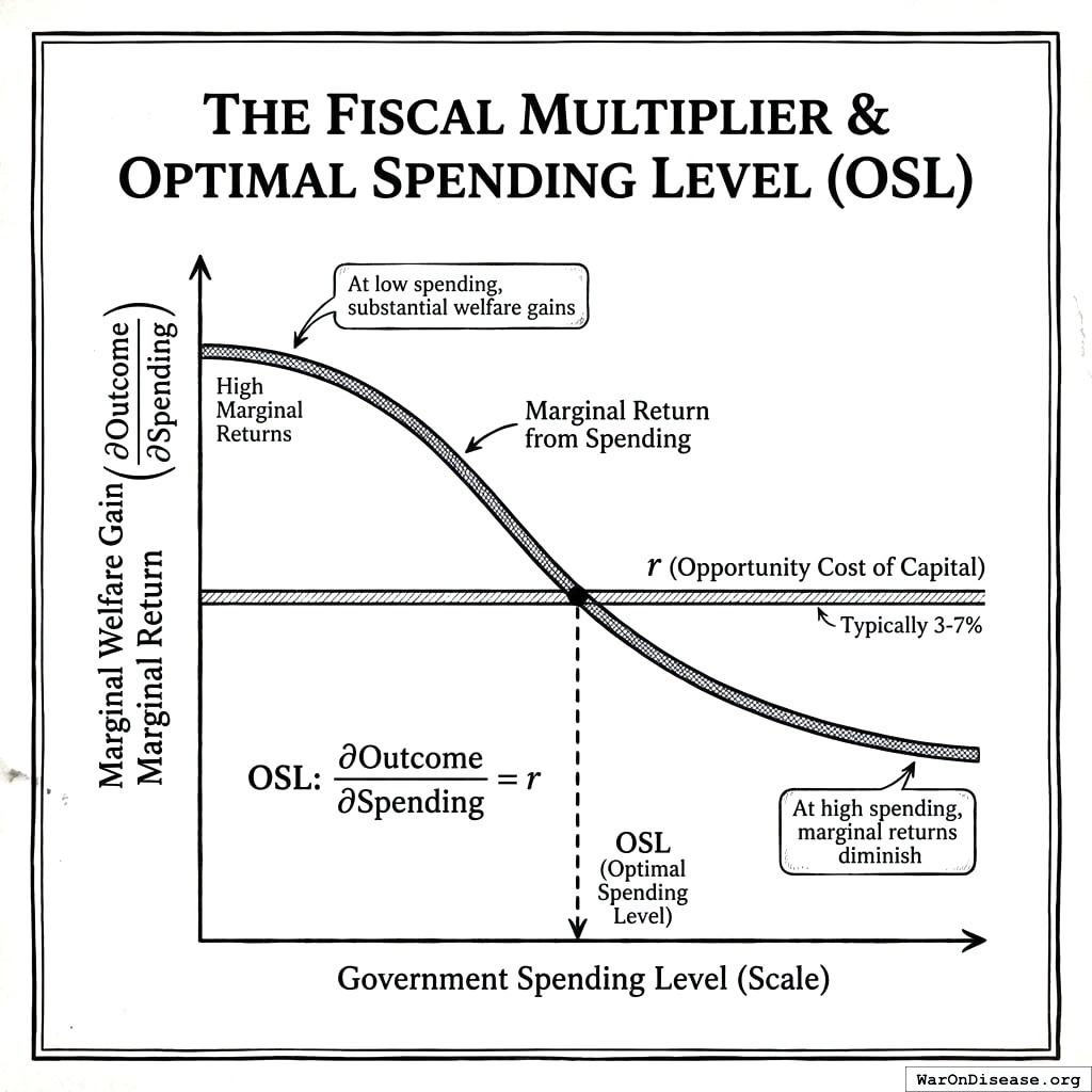
\[ \text{OSL}: \frac{\partial \text{Outcome}}{\partial \text{Spending}} = r \]

Where \(r\) is the opportunity cost of public funds: the marginal welfare \(\lambda^*\) of the best alternative use of the last dollar (another goal, the universal cash payment, or lower taxes).

Finding the “Knee” of the Curve

Empirically, we look for the point where the outcome-spending relationship flattens:

Outcome
   ^
   |                    ___________
   |                 __/
   |               _/
   |             _/
   |           _/   <- OSL is around here
   |         _/
   |       _/
   |     _/
   |   _/
   | _/
   |/
   +-----------------------------------> Spending
         Low            High

Estimation Methods

1. Nonlinear regression on cross-country data

Fit diminishing returns functions:

\[ \text{Outcome} = \alpha + \beta \cdot \log(\text{Spending}) + \epsilon \]

Or with saturation:

\[ \text{Outcome} = \alpha + \beta \cdot \frac{\text{Spending}}{\text{Spending} + \gamma} \]

Where \(\gamma\) is the half-saturation constant.

2. Piecewise linear estimation

Estimate separate slopes for different spending ranges to identify where returns diminish.

3. Meta-regression of effect estimates

If multiple studies estimate effects at different spending levels, meta-regression can identify how effects vary with baseline spending. The credibility of such estimates depends critically on identification strategy⁴².

Worked Example: K-12 Education Spending

Primary metric affected: Real after-tax median income growth (via higher wages from improved skills).

⁴³ exploited court-ordered school finance reforms to estimate causal effects of K-12 spending. Key finding: a 10% increase in per-pupil spending increases adult earnings by 7% for students from low-income families.

Does this effect diminish at higher spending levels?

Evidence from cross-state variation suggests:

Baseline spending (per pupil)	Effect of 10% increase	Implied marginal return
$8,000	+8% earnings	$0.80 per $1
$12,000	+5% earnings	$0.50 per $1
$16,000	+3% earnings	$0.30 per $1
$20,000	+1% earnings	$0.10 per $1

OBG estimation: At $16,000/pupil, the marginal return (~0.30) roughly equals the social discount rate. This suggests:

• Current US average: ~$15,000/pupil
• OSL: ~$16,000-$18,000/pupil (modest underinvestment)
• Gap: ~$50B nationally

Evidence grade: B (strong causal identification, moderate extrapolation uncertainty)

Worked Example: Pragmatic Clinical Trials

The Highest-Return Public Investment

Metrics affected: Both real after-tax median income growth (via reduced healthcare costs and improved productivity) and median healthy life years (via better treatments). This dual impact contributes to the exceptionally high returns.

Some ways of spending government money work better than others. Also, cheap trials work as well as expensive trials, but cost less. This required two charts to explain.

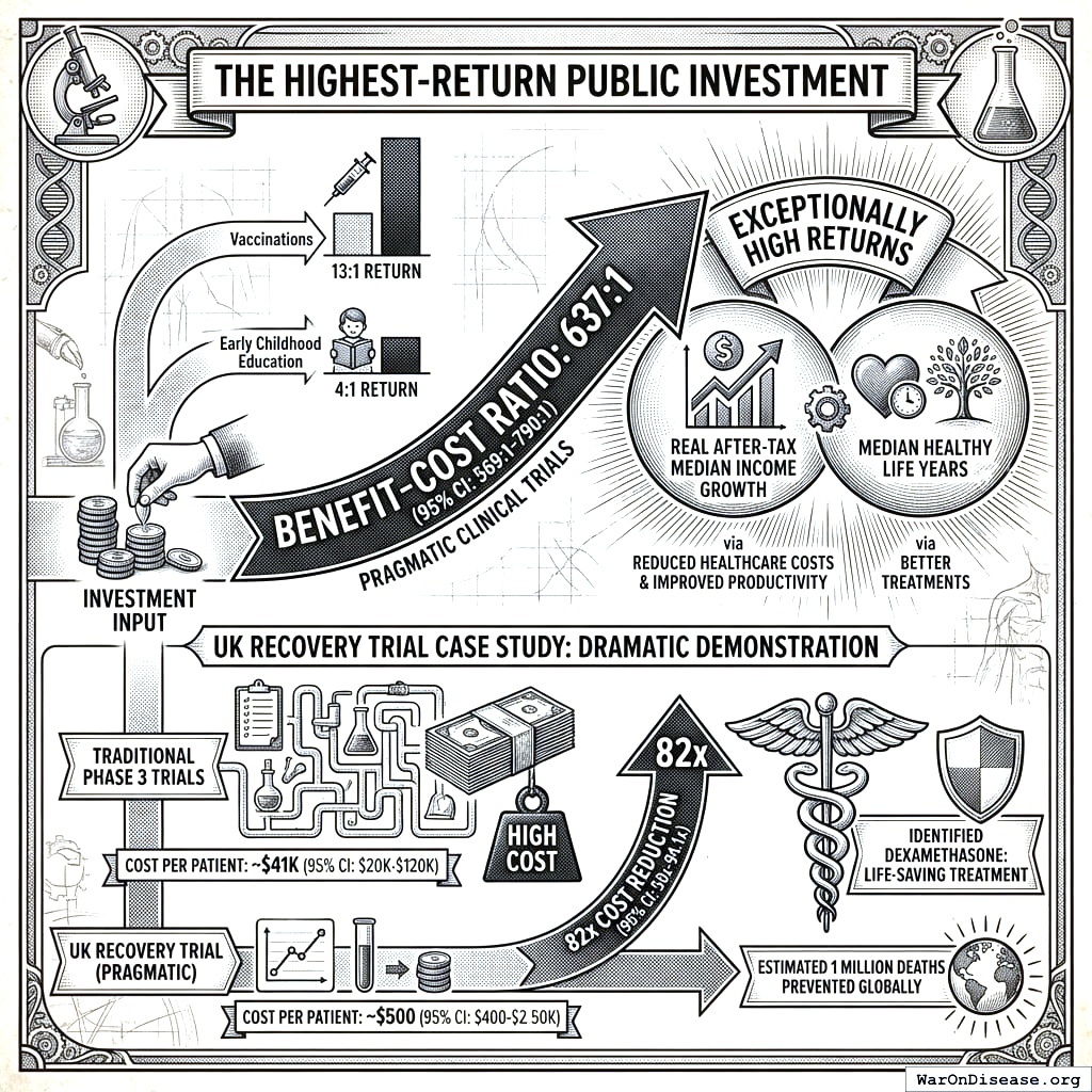
Pragmatic clinical trials represent perhaps the single highest-return category of public investment identified in the literature. While vaccinations return 10.9:1 and early childhood education returns 4:1, pragmatic trials demonstrate benefit-cost ratios of 439 (90% CI: 321-600):1⁴⁴.

The UK’s RECOVERY trial demonstrated this dramatically during COVID-19: it cost approximately $500 (95% CI: $400-$2,500) versus $41,000 (95% CI: $20,000-$120,000) for traditional Phase 3 trials, a 82x (90% CI: 21.4x-195x) cost reduction⁴⁵. This single trial identified dexamethasone as a life-saving treatment, preventing an estimated 1 million deaths globally.

OSL Estimation

Pragmatic trials represent an innovation frontier where no country has achieved optimal investment. We estimate OSL from cost-effectiveness analysis:

1. Unmet medical need: Approximately 2.88 billion DALYs/year (90% CI: 2.63 billion DALYs/year-3.12 billion DALYs/year) from conditions lacking adequate treatment
2. Cost per DALY averted: Pragmatic trials cost $929 (95% CI: $929-$1,400) (ADAPTABLE trial) vs. $41,000 (95% CI: $20,000-$120,000) traditional
3. Scale-up potential: Current global clinical trial spending is approximately $60 billion (95% CI: $50 billion-$75 billion)/year, but only ~$500M goes to pragmatic/embedded designs

Data Point	Value	Source
Current pragmatic trial spending (US)	~$500M	NIH Common Fund
Traditional trial spending (global)	$60 billion (95% CI: $50 billion-$75 billion)	Industry + NIH
Cost per patient (pragmatic)	$929 (95% CI: $929-$1,400)	ADAPTABLE trial
Cost per patient (traditional Phase 3)	$41,000 (95% CI: $20,000-$120,000)	Industry average
Cost reduction factor	44.1x (90% CI: 12.8x-210x)	Calculated

Diminishing Returns Analysis

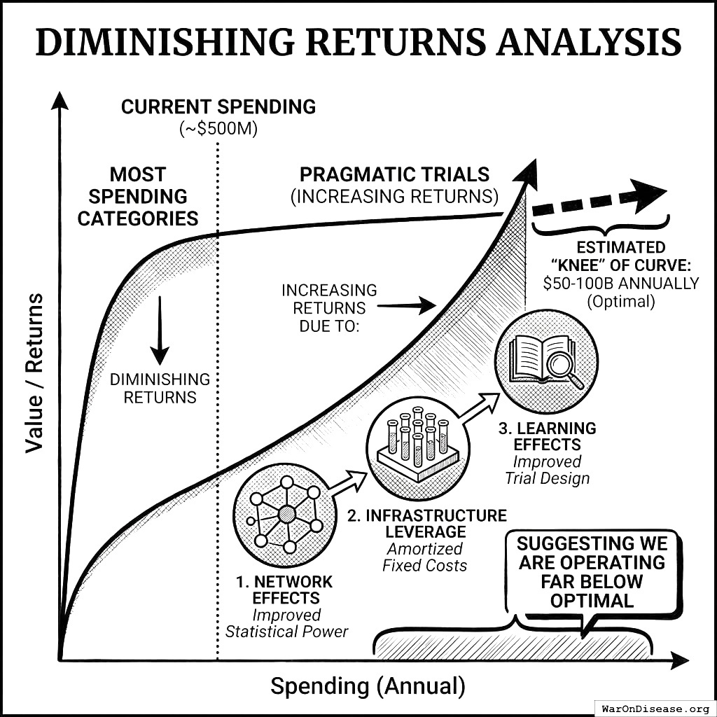
Unlike most spending categories, pragmatic trials show increasing returns at current spending levels due to:

1. Network effects: Each additional participant improves statistical power for all trials
2. Infrastructure leverage: Platform trials amortize fixed costs across multiple interventions
3. Learning effects: Evidence accumulation improves trial design efficiency

The “knee” of the diminishing returns curve is estimated at $50-100B annually (vs. current ~$500M), suggesting we are operating far below optimal.

We spend 500 million on pragmatic trials. The graph says we should spend 50 to 100 billion. We are so far to the left of where we should be that we’re practically off the chart.

Cost-Effectiveness Calculation

Using standard health economics methodology:

Component	Value	Calculation
Cost per pragmatic trial participant	$929 (95% CI: $929-$1,400)	ADAPTABLE benchmark
QALYs gained per participant	0.05-0.2	Evidence generation value
Cost per QALY	$4,600-$18,600	Well below $50K threshold
Scale-up population	50M patients/year	10% of treatable conditions
OSL estimate	$50B/year	Conservative

Gap Analysis

Metric	Value
Current spending (pragmatic trials)	~$500M
OSL	$50B
Gap	+$49.5B (99x underinvestment)
Gap % of current	+9,900%
Opportunity cost	439 (90% CI: 321-600):1 foregone returns

Evidence grade: A (RCT evidence from RECOVERY, ADAPTABLE; strong theoretical foundation)

Why This Category Dominates

Pragmatic clinical trials have the highest priority score of any analyzed category that needs more money:

\[ \text{Priority} = |\text{Gap}| \times \text{BIS} = \$49.5B \times 0.90 = 44.6 \]

The only other derived increase, vaccinations, scores 7.6. Basic research and early childhood have strong evidence that more spending helps, but their OSLs are not derived yet, so they have no priority score. Military spending has a larger absolute priority score (351) because its gap is large, but it is overinvestment that requires a cut.

Cost-Effectiveness Threshold Analysis

The Standard Health Economics Approach

Cost-effectiveness analysis has become the standard framework for health resource allocation decisions¹¹. The QALY (Quality-Adjusted Life Year) puts every health intervention in the same unit, so costs per QALY can be compared with each other and against a willingness-to-pay threshold^11,39.

For health interventions, cost-effectiveness analysis provides OSL estimates:

\[ \text{OSL} = \sum_{\text{interventions}} \text{Scale}_i \times \text{Cost}_i \quad \text{where } \frac{\text{Cost}_i}{\text{QALY}_i} < \text{WTP} \]

Where:

• \(\text{Scale}_i\) = target population for intervention \(i\)
• \(\text{Cost}_i\) = per-person cost of intervention \(i\)
• \(\text{QALY}_i\) = QALYs gained per person from intervention \(i\)
• \(\text{WTP}\) = willingness-to-pay threshold (typically $50K-$150K per QALY)

Building Up from Intervention-Level Data

Four boxes with arrows between them. The boxes show how you take lots of small numbers and turn them into one big number. Addition with extra steps.

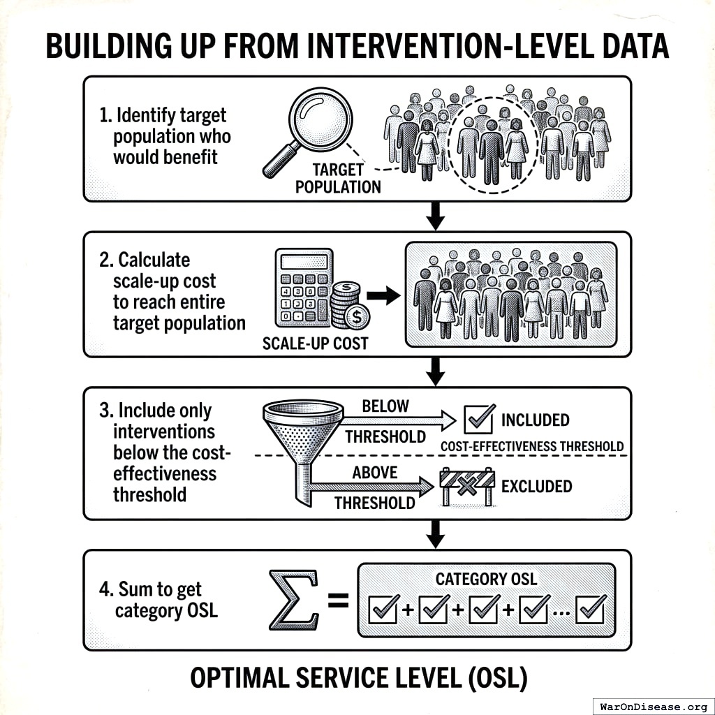
For each health intervention with cost-effectiveness data:

1. Identify target population who would benefit
2. Calculate scale-up cost to reach entire target population
3. Include only interventions below the cost-effectiveness threshold
4. Sum to get category OSL

Worked Example: Vaccinations

Primary metric affected: Median healthy life years (via disease prevention and mortality reduction).

Vaccinations are among the highest-return public health investments. Routine US childhood immunization returns about 10.9:1, counting medical and productivity savings⁴⁶. Across 94 low- and middle-income countries, the return is about 44:1 when the value of longer, healthier lives is counted⁴⁷, and about 101:1 for reaching the children still missed in 80 of the poorest countries by 2030⁴⁸. The poorer the country and the more of a life the analysis counts, the larger the ratio.

Cost-effectiveness estimates from CEA Registry and CDC vaccination cost studies. QALY estimates reflect average health gains across target populations; costs include vaccine acquisition, administration, and program overhead.

Intervention	Target pop.	Cost/person	QALY/person	Cost/QALY	Source	Include?
Childhood routine	4M births	$500	0.1	$5,000	CDC VFC	Yes
HPV vaccination	4M teens	$300	0.05	$6,000	CEA Registry	Yes
Flu (elderly)	50M elderly	$40	0.01	$4,000	CDC	Yes
Shingles	40M eligible	$200	0.02	$10,000	CEA Registry	Yes
COVID boosters	100M adults	$30	0.005	$6,000	CDC	Yes

All interventions fall well below the conventional $50,000-$150,000 per QALY cost-effectiveness threshold, indicating strong economic justification for full scale-up.

OBG calculation:

• Childhood routine: 4M × $500 = $2.0B
• HPV: 4M × $300 = $1.2B
• Flu (elderly): 50M × $40 = $2.0B
• Shingles: 40M × $200 = $8.0B
• COVID boosters: 100M × $30 = $3.0B
• Total OSL: ~$16B (vs. current ~$8B)

Gap: +$8B (underinvestment)

Evidence grade: A (RCT evidence for most vaccines, well-established cost-effectiveness)

Efficiency Frontier Analysis

Waste Versus Diminishing Returns

A dose-response curve fitted through every jurisdiction’s spending and outcomes describes the average government. The average government wastes some of its money, so the average curve mixes two different things: waste and diminishing returns. An efficiency frontier separates them. It traces the most output that any jurisdiction gets at each spending level, with data envelopment analysis³⁰ or stochastic frontier analysis³¹.

The frontier splits each category’s gap into two parts:

1. Waste. This is the distance from a jurisdiction to the frontier. The jurisdiction can remove it by producing the same output at lower cost. Across 20 OECD countries in 2009-2013, the average waste was 26.8% of public spending, and only Switzerland was on the frontier⁴⁹.
2. Reallocation. This is the move along the frontier until the marginal return equals the opportunity cost \(\lambda^*\).

The slope of the frontier at each spending level is the best attainable marginal return, which is the \(f_{im}'\) that Proposition 1 needs. OBG therefore fits dose-response curves to the frontier, not to the average.

Health care is the clearest case. In 2016 the United States spent 17.8% of GDP on health care and ten other high-income countries spent 9.6% to 12.4%, yet US life expectancy was the lowest of the 11 countries and US infant mortality was the highest¹³. Most of the US gap is distance to the frontier, not a shortage of spending.

Limits. Frontier estimates show correlation, not cause. They are sensitive to outliers and to errors in measured output, and jurisdictions differ in need. An OSL from a frontier alone has a BIS of at most 0.59 until causal evidence on returns supports it.

Worked Example: Military Spending as a Cost Frontier

A cross-country frontier works poorly for defense: few countries face the same threats, and security has no single measured output. Peer spending is also a poor guide, for three reasons:

1. A share of GDP measures the economy, not the threat. A target set as a percentage of GDP assumes that defense needs grow with the economy. The threats that defense answers do not grow when the economy grows (The Eisenhower Curve).
2. Allied spending is not independent. Smaller alliance members spend a smaller share of income on defense because they benefit from the defense that larger members provide⁵⁰. Their spending responds to US spending, so it cannot measure what US defense requires.
3. Peer spending records an arms race. Each country’s spending rises with its rivals’ spending (see Goals whose value depends on rivals). Copying the equilibrium copies the race.

OBG therefore builds a cost frontier: the least cost, at efficient prices, of each capability that defending the country’s residents requires.

Threat	Least-cost capability	Annual cost
Strategic nuclear attack	Survivable second strike	$30 billion (95% CI: $20 billion-$50 billion)
Air and missile attack on the homeland	Continental air and missile defense, early warning	$35 billion (95% CI: $25 billion-$50 billion)
Maritime and coastal threats	Coast Guard	$14 billion (95% CI: $12 billion-$16 billion)
Territorial defense and disaster response	National Guard	$30 billion (95% CI: $24 billion-$40 billion)
Cyberattack on critical infrastructure	Cyber defense	$15 billion (95% CI: $10 billion-$25 billion)
A peer threat that has not emerged yet	Mobilization hedge: defense R&D, industrial base, professional cadre	$60 billion (95% CI: $40 billion-$100 billion)
Cost frontier for defending the United States		$184 billion (90% CI: $158 billion-$215 billion)

The threat list and the cost of each line are derived in The Eisenhower Curve. The FY2024 US military budget (defense discretionary budget authority) is $886 billion⁵¹, so reaching the cost frontier is a cut of $702 billion (90% CI: $671 billion-$728 billion) (79.2% (90% CI: 75.7%-82.2%)). The comparison is budget to budget; actual FY2024 national defense outlays were $874.0 billion⁵², which would lower the cut by about $12 billion.

Why the higher published figures are not the OSL. Restraint proposals and peer benchmarks scaled to US GDP give roughly $450-675 billion (The Eisenhower Curve). Those figures buy a larger output: a reduced version of the US role in defending other countries. OBG’s welfare function counts the median income and healthy life years of the country’s own residents, so defending other countries counts only through its effect on the risk to those residents. That extra output is in the OSL only if its marginal welfare per dollar beats \(\lambda^*\), and the cost-benefit ledger of hegemony argues that it does not.

Evidence grade: C. The capability costs are stated assumptions, not causal estimates of the return to each dollar, so BIS is 0.50.

Delivery Methods and the Cash Benchmark

A spending category names a goal, not a method. For each goal, OBG compares the delivery methods that could reach it and funds the one with the highest marginal welfare per dollar (Proposition 1).

Delivery method	Example	Tends to work best when	Evidence example
Direct public provision	Public vaccination programs	The good is shared (herd immunity, clean air)	Vaccination worked example
Vouchers	School vouchers	Depends on design and setting	Louisiana’s statewide voucher lowered participants’ math scores by 0.4 standard deviations in the first year53; Washington, DC’s voucher raised high school graduation from 70% to 82%54
Cash transfers	Unconditional cash	People can buy what they need themselves	Associated with about 20% lower mortality among adult women and 8% lower among children under five in 37 countries55
Prizes and advance purchase commitments	Pneumococcal vaccine commitment	A new product is needed and research is uncertain	56
Payment for results	Outcome contracts, Incentive Alignment Bonds	The outcome is easy to measure	3
Rule changes	Licensing or approval reform	A rule blocks the goal	See the Optimal Policy Generator2

The Cash Benchmark

Cash benchmarking compares a program with giving its cost to the intended beneficiaries in cash⁵⁷. In a Rwandan youth employment trial, cost-equivalent cash improved more economic outcomes than USAID-funded job training⁵⁷. OBG applies the same test to every delivery method: a method gets money only if its marginal welfare per dollar beats cash.

Cash does not always win. In US data, direct investments in low-income children’s health and education have the highest marginal value of public funds of any policy type, and many pay for themselves⁵⁸. The Happier Lives Institute estimates that two lay-delivered psychotherapy programs produce about 40 to 49 WELLBYs per $1,000, five to six times its estimate for cash transfers, although the only randomized trial of one of them found much smaller effects⁵⁹. Some goals cannot be bought with cash at all. Basic research, clean air, herd immunity, and pragmatic trials are shared goods: no individual buys them with a cash payment. For those goals, the comparison is among public provision, prizes, and payment for results.

To compare methods in one unit, OBG converts each method’s effects to the standardized two-metric welfare units. Where studies report it, OBG also records the marginal value of public funds, a benefit-cost ratio that includes a policy’s effect on government revenue^58,60.

Universal Cash Payment as a Budget Category

A universal cash payment (for example, a universal basic income) is a budget category with its own diminishing-returns curve. Each extra dollar is worth less to the same person, and the cost of a universal payment grows with the population. The evidence on cash transfers so far:

Outcome	Finding	Setting
Mortality	About 20% lower for adult women and 8% lower for children under five, in an observational difference-in-differences analysis55	37 low- and middle-income countries
Consumption and well-being	Higher household consumption and large gains in psychological well-being nine months later61	Randomized trial, rural Kenya
Local economy	Each dollar raised local economic activity by about $2.5, with minimal price inflation62. This is a local multiplier in a poor rural economy and does not apply as-is to a national payment in a rich country	Randomized trial, rural Kenya
Work	No systematic evidence that transfers discouraged work63	7 randomized trials, 6 developing countries
Work	No detectable effect on overall employment; part-time work rose 1.8 percentage points64	Alaska Permanent Fund Dividend
Work and well-being	Employment rose slightly (about 6 extra days over one year), and recipients reported better well-being on several measures65	Randomized experiment, 2,000 unemployed people, Finland
Work	$1,000 a month for three years reduced work by about 1 to 2 hours a week and labor market participation by about 4 percentage points66	Randomized trial, Texas and Illinois (working paper)

OBG estimates the cash payment’s OSL like any other category: it is the level where the payment’s marginal welfare equals the marginal cost of raising the revenue (Proposition 1). The illustrative example in this paper does not estimate this curve yet.

Lower Taxes as the Final Benchmark

Every dollar of spending must first be raised. The marginal cost of public funds measures the loss to society from raising an additional dollar of government revenue³⁴. When it exceeds one, each dollar of spending costs society more than a dollar. OBG includes this cost as \(C(B)\) in the planner’s problem. If no use of money, including the universal cash payment, beats \(C'(B)\), the optimal budget is smaller and the money stays with taxpayers. The welfare effect of a tax cut can be measured the same way as a program’s, through its marginal value of public funds⁶⁰.

A universal cash payment and a tax cut both return money to people, but to different people. A flat payment gives the same amount to everyone, while a tax cut returns more to those who pay more tax. Because OBG optimizes median income and median healthy life years, it weighs these two options differently, and the data decide between them.

Budget Impact Score (BIS)

The Budget Impact Score measures confidence in each category’s OSL estimate based on the quality and quantity of causal evidence. The scoring methodology draws on the established evidence hierarchy from the econometrics literature^42,67.

A pyramid of trustworthiness. Randomized trials sit at the top wearing a crown. Someone’s opinion sits at the bottom, wondering what it did wrong.

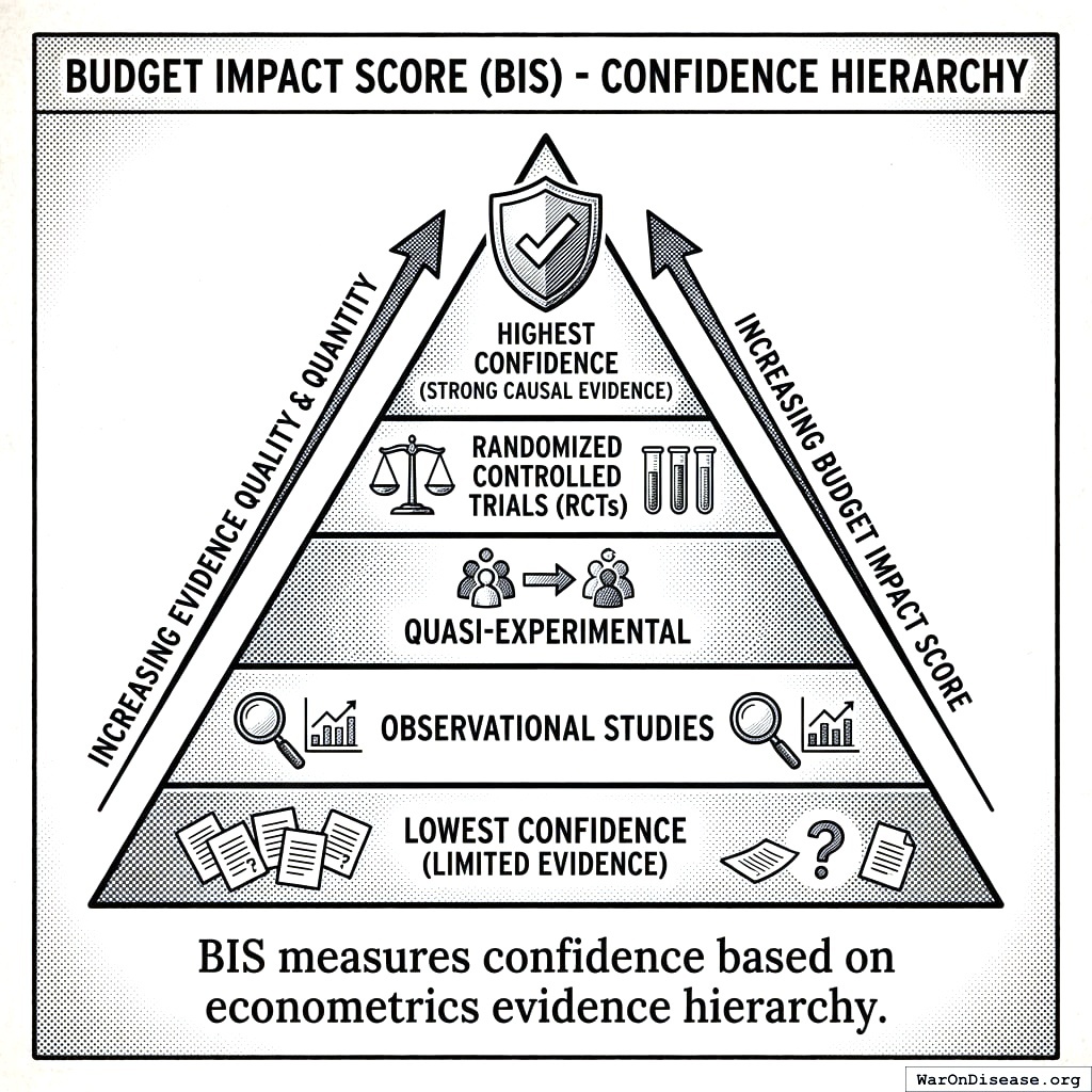
BIS Calculation

For each spending category \(i\):

Step 1: Gather effect estimates

Collect all available causal effect estimates \(\{\beta_{i,1}, \beta_{i,2}, ..., \beta_{i,n_i}\}\) from the econometric literature.

Step 2: Compute quality weights

Identification Method	Quality Weight (\(w^Q\))
Randomized controlled trial	1.00
Natural experiment (difference-in-differences, regression discontinuity)	0.85
Instrumental variables	0.70
Panel with fixed effects	0.55
Cross-sectional regression	0.25

Step 3: Compute precision weights

\[ w^P_j = \frac{1}{\text{SE}(\beta_j)^2} \]

Step 4: Compute recency weights

\[ w^R_j = e^{-0.03(t_{now} - t_j)} \]

Step 5: Compute confidence score

\[ \text{BIS}_i = \min\left(1, \frac{\sum_j w^Q_j \cdot w^P_j \cdot w^R_j}{K}\right) \]

Where \(K\) is a calibration constant.

Evidence Grading from BIS

BIS Range	Grade	Interpretation	OSL Confidence
0.80 - 1.00	A	Strong causal evidence	High - proceed with reallocation
0.60 - 0.79	B	Good evidence	Moderate - proceed with monitoring
0.40 - 0.59	C	Mixed evidence	Low - pilot before scaling
0.20 - 0.39	D	Weak evidence	Very low - research priority
0.00 - 0.19	F	Insufficient evidence	Unknown - cannot estimate OSL

Gap Analysis and Priority Ranking

Computing Gaps

For each category \(i\):

\[ \text{Gap}_i = \text{OSL}_i - \text{Current}_i \]

• Gap > 0: Underinvestment (increase spending)
• Gap = 0: At optimal (maintain)
• Gap < 0: Overinvestment (decrease spending)

Priority Score

Prioritize reallocation by gap size weighted by confidence:

\[ \text{Priority}_i = |\text{Gap}_i| \times \text{BIS}_i \]

Categories with large gaps AND high confidence should be addressed first.

Illustrative Example: Priority Ranking

The following uses the same illustrative data from the dashboard example above. OSL estimates for pragmatic trials and vaccinations come from the worked examples in this paper, and the military OSL comes from the threat-based cost frontier. The agricultural subsidy OSL comes from the cash benchmark: a payment to one industry must beat giving the same dollar to everyone as cash. The example assumes that farm payments fail this test; the zero is an assumption until the payments’ returns are estimated. BIS scores summarize available causal evidence quality.

Category	Current	OSL	Gap	BIS	Inc	Hlth	Priority	Action
Military	$886 billion	$184 billion (90% CI: $158 billion-$215 billion)	Cut $702 billion (90% CI: $671 billion-$728 billion)	0.50	−	−	351	Decrease
Pragmatic trials	$0.5B	$50B	+$49.5B	0.90	++	+++	44.6	Scale 100x
Ag subsidies	$25B	$0B	-$25B	0.59	−	−	14.8	Eliminate
Vaccinations	$8B	$16B	+$8B	0.95	+	+++	7.6	Increase
Basic research	$45B	Not derived	Not derived		++	++	None	Estimate OSL
Early childhood	$50B	Not derived	Not derived		+++	+	None	Estimate OSL

Inc = effect on real after-tax median income growth. Hlth = effect on median healthy life years. Scale: +++ strong, ++ moderate, + weak, − negative. The military priority uses the central gap of about $702B.

Reallocation plan: Cut military spending by $702 billion (90% CI: $671 billion-$728 billion) and agricultural subsidies by $25B, and fund pragmatic clinical trials (+$49.5B) and vaccinations (+$8B). The cuts are much larger than the increases. The difference goes to its highest-value use under Proposition 1: categories whose OSLs are not derived yet (basic research and early childhood have the strongest evidence of benefit; see Appendix C), a universal cash payment, or lower taxes. This example does not estimate those marginal values yet, so it leaves the difference unassigned rather than choosing a use arbitrarily. Among the derived increases, pragmatic trials have the highest priority score because of extreme underinvestment combined with strong evidence, and they improve both welfare metrics.

Multi-Unit Reporting

The Problem with Abstract Scores

Composite scores (like 0-1 BIS values) obscure interpretability. Policymakers and citizens understand dollars, lives, and years - not abstract indices.

Reporting at Multiple Levels

Level	Units	Use Case	Example
0. Core metrics	pp/year income growth, healthy life years	Primary welfare outcomes	“+0.1 pp income growth, +0.05 healthy years”
1. Natural	Domain-specific	Interpretation within domain	“Education: $2,100/student gap”
2. Monetized	$ equivalent	Cross-domain comparison	“Expected welfare gain: $4.00 per $1”
3. Health	QALYs/DALYs	Health-weighted comparison	“12,000 QALYs per $1B invested”
4. Composite	0-1 score	Ranking when monetization uncertain	“BIS = 0.85”

Level 0 (Core Metrics) reports expected changes to the two welfare metrics directly. All other levels are derived from or convertible to these core outcomes. QALYs (Level 3) translate directly to median healthy life years. Monetized values (Level 2) combine income effects with health effects valued at standard rates.

Conversion Factors

Conversion	Value	Source	Notes
Value of Statistical Life (VSL)	~$10M	EPA, DOT	US regulatory standard
Value per QALY	$50K-$150K	ICER, WHO	Context-dependent
QALY → $	$100K/QALY	Mid-range estimate	For cross-domain
Life-year → QALY	~0.8-1.0	Age/health adjusted	Quality weighting

Worked Example: Multi-Unit Output

Category: Early Childhood Education (a hypothetical $20B increase; the OSL is not derived)

Unit Level	Value	Interpretation
Natural	+$20B increase	Current: $50B; OSL not derived
Per-child	+$833/child	24M children
Monetized ROI	~4:1 benefit-cost (5% discount, conservative crime costs); 7-10% annual social return	68
Health (QALYs)	+8K QALYs/year	Per $1B additional
Composite (BIS)	Not graded	Randomized evidence of effects (small samples), but no derived OSL

Recommendation: The evidence that more spending helps is strong; the level where returns fall to the opportunity cost is not derived. If Perry-level returns held at national scale, a $20B increase would yield about $80B in discounted benefits, about $60B net of cost.

Quality Requirements and Validation

Minimum Thresholds for OBG Estimation

Criterion	Minimum	Rationale
Reference countries	5+	Avoid outlier bias
Dose-response studies	3+	Identify diminishing returns
Causal effect estimates	2+	Cross-validate
Data recency	Within 10 years	Relevance
BIS for reallocation	> 0.40	Sufficient confidence

Robustness Checks

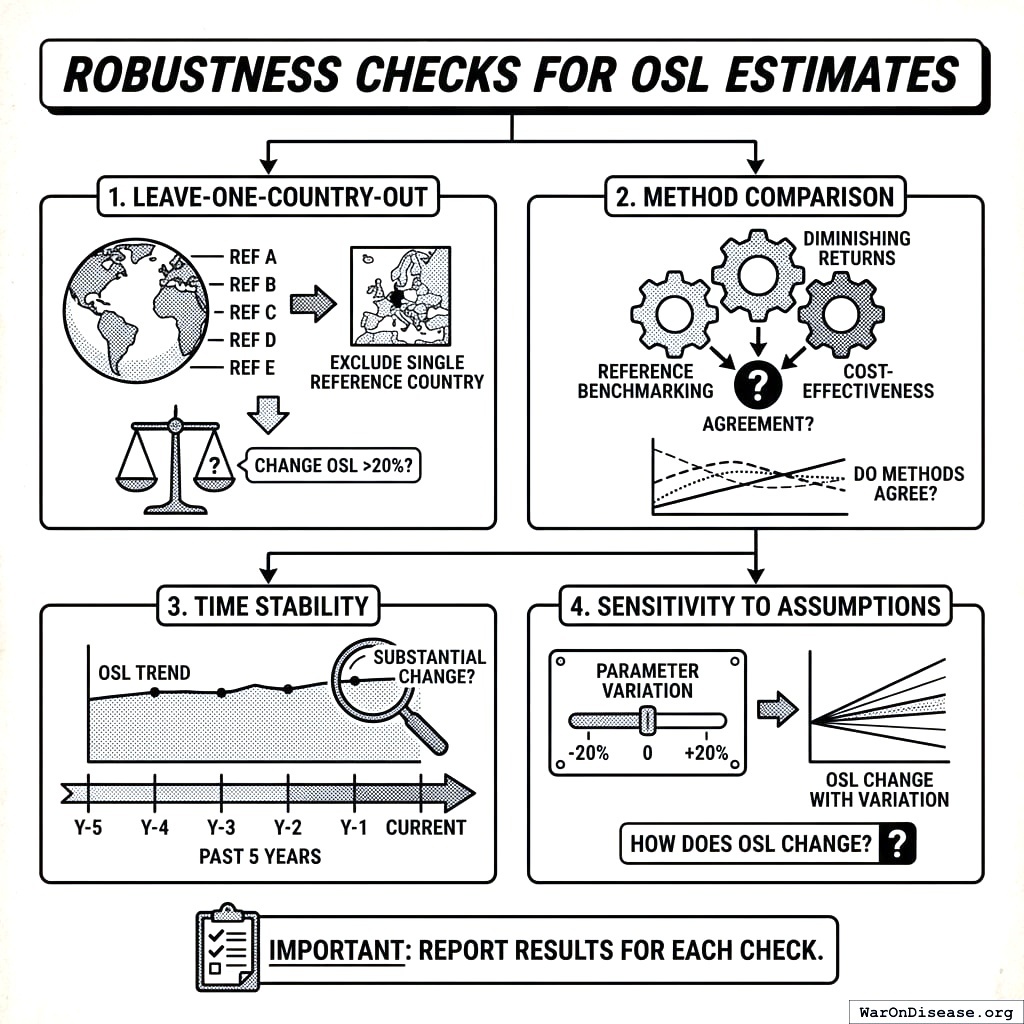
For each OSL estimate, report:

1. Leave-one-country-out: Does excluding any single country change OSL by >20%?
2. Method comparison: Do diminishing returns and cost-effectiveness methods agree?
3. Time stability: Has OSL changed substantially over past 5 years?
4. Sensitivity to assumptions: How does OSL change with ±20% parameter variation?

Four ways to check if your answer is wrong. Look for weird numbers. Make sure you did the same thing every time. Check if it changes when time passes. Wiggle the inputs and see if it explodes.

Interpreting Results

Gap Ranges and Recommended Actions

Gap (% of current)	Interpretation	Recommended Action
> +50%	Severe underinvestment	Immediate scale-up
+20% to +50%	Moderate underinvestment	Phased increase
-10% to +20%	Near optimal	Monitor, fine-tune
-50% to -10%	Moderate overinvestment	Gradual reduction
< -50%	Severe overinvestment	Urgent reallocation

What the Algorithm Cannot Tell You

Factor	OBG Captures	OBG Does Not Capture
Evidence-optimal spending level	Yes
Confidence in estimates	Yes
Direction of reallocation	Yes
Political feasibility		No
Implementation capacity		No
Transition costs		No
Distributional effects		No
Novel interventions		No

OBG provides evidence-based targets. Political judgment is still required for implementation strategy.

Pilot Program Prioritization

Value of Information for Uncertain Categories

Categories with low BIS but potentially high returns warrant research investment:

\[ \text{VOI}_i = \text{Potential Gap}_i \times (1 - \text{BIS}_i) \times P(\text{high return}) \]

High-VOI categories should receive pilot funding to generate better evidence.

Recommended Pilot Designs

Four ways to test if your idea works before spending billions. Option 1: flip a coin. Option 2: do it slowly. Option 3: wait for something to happen and watch. Option 4: check if someone already wrote it down.

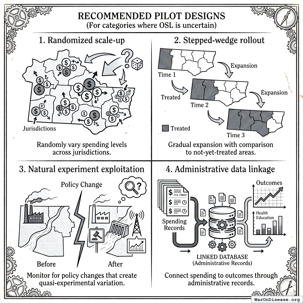
For categories where OSL is uncertain:

1. Randomized scale-up: Randomly vary spending levels across jurisdictions
2. Stepped-wedge rollout: Gradual expansion with comparison to not-yet-treated areas
3. Natural experiment exploitation: Monitor for policy changes that create quasi-experimental variation
4. Administrative data linkage: Connect spending to outcomes through administrative records

Learning Feedback Loop

A circle with four boxes in it. The boxes say: spend money, see what happened, learn from it, spend money differently. Then you go around the circle again. It’s like learning from your mistakes, but on purpose.

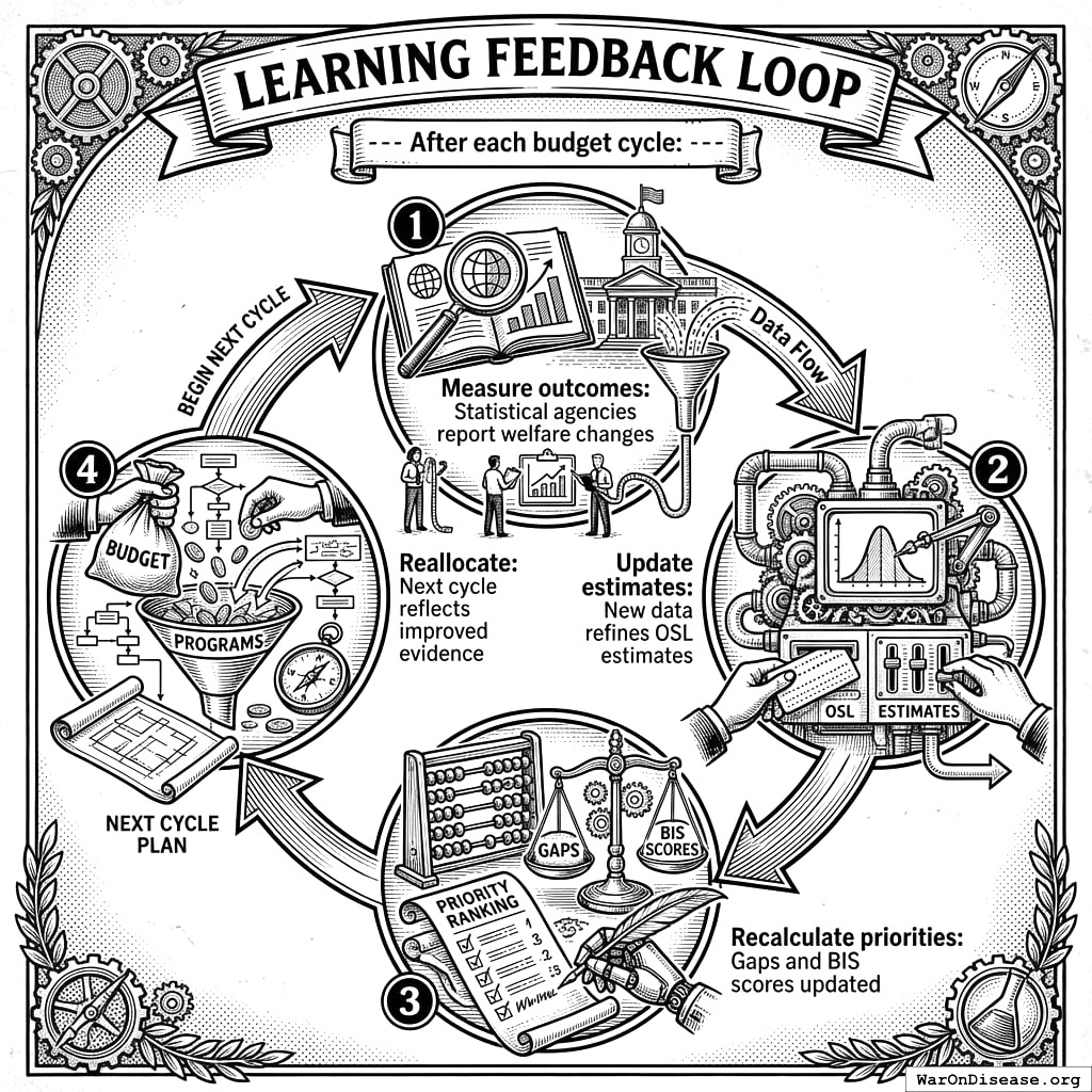
After each budget cycle:

1. Measure outcomes: Statistical agencies report welfare changes
2. Update estimates: New data refines OSL estimates
3. Recalculate priorities: Gaps and BIS scores updated
4. Reallocate: Next cycle reflects improved evidence

Data Sources

Cross-Country Databases

International organizations maintain standardized cross-country spending and outcome data essential for diminishing returns analysis. The OECD provides the most comprehensive harmonized data for high-income countries¹².

Database	Coverage	URL	Use Case
OECD iLibrary	38 OECD members	oecd-ilibrary.org69	Education, health, social spending
World Bank WDI	217 countries	data.worldbank.org70	Broad spending and outcomes
SIPRI	Global	sipri.org71	Military spending
WHO GHED	194 countries	who.int/data/gho72	Health expenditure
UNESCO UIS	Global	uis.unesco.org73	Education spending

Cost-Effectiveness Databases

Database	Coverage	URL	Use Case
CEA Registry	8,000+ analyses	cearegistry.org74	Health cost-effectiveness
Disease Control Priorities	LMICs	dcp-3.org75	Global health priorities
Cochrane Library	8,000+ reviews	cochranelibrary.com76	Health intervention effects
Copenhagen Consensus	Development	copenhagenconsensus.com77	Development priorities

These databases enable systematic ranking of interventions by cost-effectiveness. For example, GiveWell’s 2011 analysis, which it now marks out of date, put deworming at about $28 to $70 per DALY averted for schistosomiasis and about $83 for soil-transmitted worms; GiveWell now judges deworming mainly by its later effect on income⁷⁸.

US Budget Data

Source	Coverage	URL	Use Case
OMB Historical Tables	1789-present	whitehouse.gov/omb79	Federal spending
CBO Budget Analyses	Federal	cbo.gov80	Fiscal impact scoring10
USASpending	Federal awards	usaspending.gov81	Program-level detail
Census of Governments	State & local	census.gov82	Subnational spending

Limitations

Diminishing Returns Uncertainty

• Functional form: True relationship may not match assumed function
• Extrapolation: Estimating returns outside observed spending range
• Interaction effects: Returns may depend on other spending categories

Mitigation: Report confidence intervals, use multiple functional forms, acknowledge extrapolation limits.

Status-Quo Bias in the Evidence Base

Most program evaluations study programs that governments already run. Delivery methods that no government has tried, or tried only at small scale, have little evidence and so receive low BIS scores. Without correction, this would bias OBG toward existing public programs. OBG corrects for it in three ways: every program must beat a universal cash payment and lower taxes, neither peer spending nor current spending can set a target, and low-evidence methods with high potential returns receive pilot funding instead of exclusion.

Mitigation: Report which OSLs are not derived, fund pilots of untried delivery methods, and update OSLs as new evidence arrives.

Implementation Capacity

Higher spending may not translate to outcomes if implementation capacity is lacking.

Money goes through two filters before it becomes results. The filters are called ‘make sure you can actually do this’ and ‘do it slowly so you don’t mess up.’ Filters for money that don’t involve coffee.

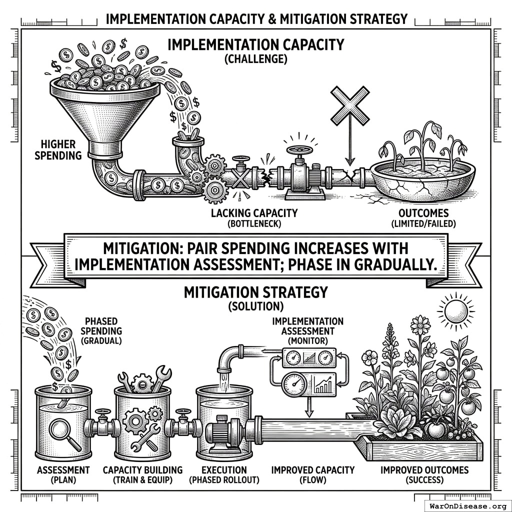
Mitigation: Pair spending increases with implementation assessment; phase in gradually.

Benchmarking Framework

This section defines how OBG should be benchmarked against historical and prospective budget outcomes.

Retrospective Validation

Question: Did jurisdictions that moved toward OSL achieve better outcomes than those that diverged?

Three steps to check if you were right. Step 1: go back in time (mathematically). Step 2: pretend you did what you should have done. Step 3: compare it to what actually happened. Like replaying a football match in your head where you win.

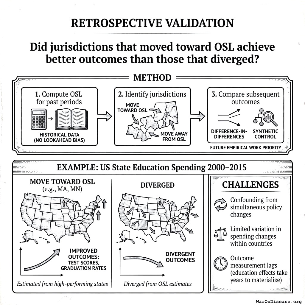
Method: 1. Compute OSL for past periods using only data available at that time (to avoid lookahead bias) 2. Identify jurisdictions that moved toward/away from OSL 3. Compare subsequent outcomes using difference-in-differences or synthetic control methods⁸³

Example: US State Education Spending 2000-2015

A retrospective analysis can examine whether states that moved toward education OSL (estimated from high-performing states like Massachusetts and Minnesota) subsequently showed improved test scores and graduation rates relative to states that diverged.

Challenges:

• Confounding from simultaneous policy changes
• Limited variation in spending changes within countries
• Outcome measurement lags (education effects take years to materialize)

Prospective Validation

Question: Do OBG-guided reallocations improve outcomes going forward?

How to prove you’re not making things up. Write down your prediction before it happens. Tell everyone. Wait. Check if you were right. It’s the scientific method for not lying to yourself.

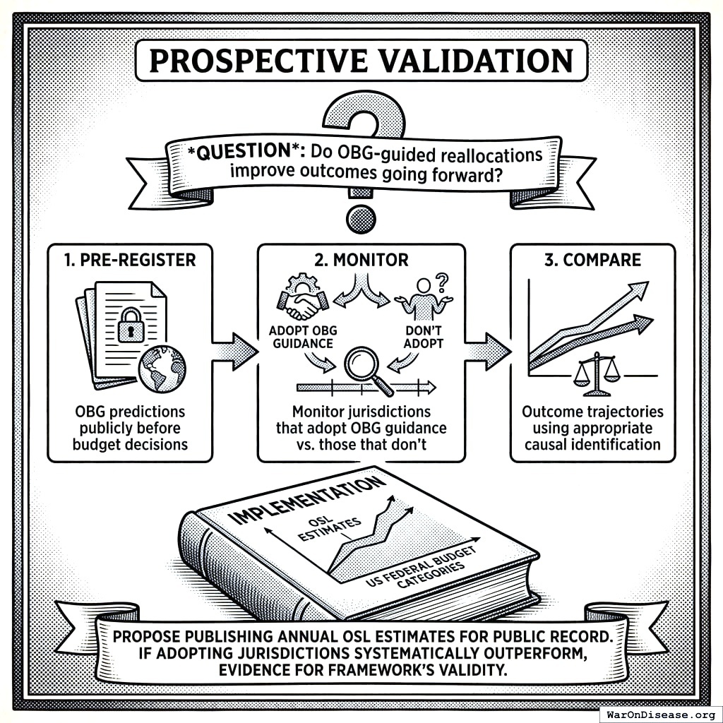
Method: 1. Pre-register OBG predictions publicly before budget decisions 2. Monitor jurisdictions that adopt OBG guidance vs. those that don’t 3. Compare outcome trajectories using appropriate causal identification

Implementation: Publish annual OSL estimates for US federal budget categories, creating a public record for prospective benchmarking. If jurisdictions that adopt OBG guidance systematically outperform those that do not, the framework is doing its job.

Success Metrics

Metric	Definition	Target	Interpretation
Gap reduction	Did spending move toward OSL?	> 50% of gap closed in 10 years	Tests political feasibility
Outcome improvement	Did welfare metrics improve more in OBG-following jurisdictions?	> 10% relative improvement	Tests welfare prediction accuracy
Prediction accuracy	Did estimated returns match actual returns?	Correlation r > 0.5	Tests underlying model
Cross-method consistency	Do diminishing returns and cost-effectiveness methods converge?	Agreement within 30%	Tests methodological robustness

Evidence Base and Benchmarking

OBG rests on the underlying studies cited throughout (e.g.,⁴³ for education,⁴⁶ and⁴⁷ for vaccinations) plus a continuous benchmarking program:

1. Data collection: Longitudinal spending and outcome data across jurisdictions
2. Historical OSL estimation: Compute past OSL using only contemporaneously available data
3. Causal analysis: Identify spending → outcome effects with strong quasi-experimental designs
4. Publication: Publish pre-registered benchmark studies and annual scorecards

Sensitivity Analysis

Parameter Sensitivity

Parameter	Default	Test Range	Impact on OSL
Country data set	All OECD	OECD + G20, High-income only	±15%
Discount rate	5%	3-7%	±20%
BIS confidence threshold	0.40	0.30-0.60	Category inclusion
Recency decay rate	0.03/year	0.01-0.05	Estimate weights

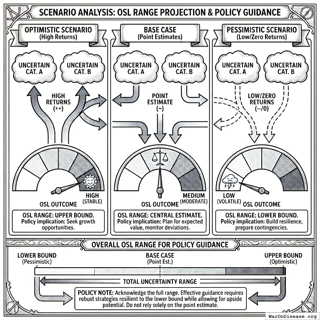
Scenario Analysis

Optimistic scenario: All uncertain categories have high returns Pessimistic scenario: Uncertain categories have low/zero returns Base case: Use point estimates

Report OSL range across scenarios for policy guidance.

Three answers to the same question. The pessimistic one assumes everything will go wrong. The optimistic one assumes everything will go right. The base case assumes you’ll be disappointed but not surprised.

Conclusion

The Optimal Budget Generator framework provides a systematic, evidence-based approach to budget allocation. Unlike marginal-return frameworks that can justify infinite spending on high-return categories, OBG recognizes that every category has an optimal level - like the Recommended Daily Allowance for nutrients.

The framework answers three questions:

1. What is the target? OBG provides evidence-based spending levels for each category
2. How far are we? Gap analysis shows where current spending diverges from optimal
3. How confident are we? BIS scores evidence quality so policymakers know which OSL estimates are reliable

Even with imperfect evidence, systematically moving from severe misallocation (in the illustrative example, military spending $702 billion (90% CI: $671 billion-$728 billion) above the cost of defending the country, and vaccinations 50% below their derived OSL) toward evidence-based targets should produce substantially larger welfare gains than current lobbying-driven allocation achieves. Because every program must beat a universal cash payment and lower taxes, those gains do not depend on keeping today’s total budget or today’s programs.

Acknowledgments

The author thanks seminar participants and anonymous reviewers for helpful comments and suggestions. All errors remain the author’s own.

Appendix A: Analysis Workflow

Complete OBG Analysis Pipeline

+-------------------------------------------------------------+
|                    OBG ANALYSIS WORKFLOW                      |
+-------------------------------------------------------------+

Phase 1: DATA COLLECTION
-------------------------
1. Budget data ingestion
   +-- Pull current spending by category (OMB, USASpending)

   +-- Normalize categories to standard taxonomy
   +-- Identify subcategories for detailed analysis
   +-- Flag data quality issues

2. Cross-country spending data
   +-- Pull spending data from OECD, World Bank
   +-- Include all comparable countries
   +-- Normalize to per-capita and % GDP
   +-- Prepare for regression analysis

3. Effect estimate data
   +-- Search systematic reviews and meta-analyses
   +-- Extract effect sizes with standard errors
   +-- Code study quality (RCT, natural experiment, etc.)
   +-- Build literature database by category

Phase 2: OSL ESTIMATION
-----------------------
4. Diminishing returns modeling
   +-- Fit nonlinear spending-outcome functions
   +-- Identify "knee" of curve
   +-- Calculate marginal returns at current spending
   +-- Estimate optimal level

5. Cost-effectiveness analysis (health/life-saving)
   +-- Identify interventions below CE threshold
   +-- Calculate scale-up costs
   +-- Sum to category OSL
   +-- Document assumptions

6. Method reconciliation
   +-- Compare OSL estimates across methods
   +-- Weight by method reliability
   +-- Produce consensus OSL estimate
   +-- Flag discrepancies

Phase 3: EVIDENCE QUALITY
-------------------------
7. BIS calculation
   +-- Compute quality weights per study
   +-- Compute precision weights
   +-- Compute recency weights
   +-- Aggregate to category BIS

8. Evidence grading
   +-- Assign A-F grade based on BIS
   +-- Document key evidence
   +-- Identify research gaps
   +-- Flag high-uncertainty categories

Phase 4: GAP ANALYSIS
---------------------
9. Compute gaps
    +-- Gap = OSL - Current
    +-- Calculate % gap
    +-- Classify as under/over/optimal
    +-- Apply BIS weighting

10. Priority ranking
    +-- Priority = |Gap| × BIS
    +-- Rank categories
    +-- Identify reallocation pairs
    +-- Estimate welfare gains

Phase 5: OUTPUT GENERATION
--------------------------
11. Multi-unit reporting
    +-- Natural units ($/capita, % GDP)
    +-- Monetized (ROI, opportunity cost)
    +-- Health units (QALYs where applicable)
    +-- Composite (BIS, evidence grade)

12. Sensitivity analysis
    +-- Vary key parameters
    +-- Test country data subsets
    +-- Report OSL ranges
    +-- Identify robust conclusions

13. Documentation
    +-- Generate category reports
    +-- Create methodology audit trail
    +-- Version control estimates
    +-- Publish to dashboard/API

Appendix B: Glossary

Core Concepts

• Optimal Budget Generator (OBG): The framework/methodology for generating integrated budget recommendations based on evidence of spending-outcome relationships. OBG chooses both the size and the composition of the budget, comparing every use of money with a universal cash payment and with lower taxes, and produces Optimal Spending Level (OSL) estimates for each goal.

You put evidence and comparison data into the machine. The machine tells you two things: how much you should spend, and how sure you should be. Then you notice you’re spending the wrong amount.

• Optimal Spending Level (OSL): The evidence-based target spending level for each category, produced by the OBG framework. \(\text{OSL}_i\) represents the optimal spending level for category \(i\). Below OSL indicates underinvestment; above OSL indicates diminishing returns.

• Budget Impact Score (BIS): A 0-1 score measuring confidence in each category’s OSL estimate based on the quality and quantity of causal evidence. Higher BIS indicates more reliable OSL recommendations.

• Spending Gap: The difference between current spending and the evidence-based target for each category. Positive gaps indicate underinvestment; negative gaps indicate overinvestment.

• Diminishing Returns: The economic principle that marginal returns to spending decrease as spending increases. The optimal level is where marginal return equals opportunity cost.

Estimation Methods

• Cost-Effectiveness Threshold: The maximum acceptable cost per QALY (or other health outcome) for including an intervention in target calculations. Typically $50K-$150K per QALY.

• Dose-Response Curve: The relationship between spending level (dose) and outcome (response). Used to identify diminishing returns and estimate optimal spending levels.

• Efficiency Frontier: The most output that any jurisdiction gets at each spending level. The distance to the frontier is waste; the frontier’s slope is the best attainable marginal return.

• Cost Frontier: The least cost, at efficient prices, of each capability a goal requires. OBG uses it for defense, where no single output can be measured across countries.

Evidence Quality

• Quality Weight (\(w^Q\)): Weight assigned to a study based on identification strategy. RCTs receive 1.0; cross-sectional studies receive 0.25.

• Precision Weight (\(w^P\)): Weight assigned based on standard error. More precise estimates receive higher weight.

• Recency Weight (\(w^R\)): Weight assigned based on publication date. More recent studies receive higher weight via exponential decay.

• Evidence Grade: Letter grade (A-F) summarizing confidence in each category’s target estimate. A = strong evidence; F = insufficient evidence.

Output Concepts

• Priority Score: Product of gap magnitude and BIS. Used to rank categories for reallocation priority.

• Value of Information (VOI): Expected benefit of additional research on uncertain categories. High-VOI categories warrant pilot funding.

• Multi-Unit Reporting: Presenting results in natural units, monetized equivalents, health units, and composite scores for interpretability.

Appendix C: Illustrative Comparison to US Budget

This appendix applies the OBG methodology to US federal budget categories as an illustrative exercise. “Current” figures are approximate FY2024 spending. The military row is FY2024 defense discretionary budget authority⁵¹; the Social Security, Medicare, Medicaid, and net interest rows are FY2024 outlays. Each OSL has a stated basis: a worked example (pragmatic trials and vaccinations), the threat-based cost frontier (military), or the cash benchmark (agricultural subsidies, as an assumption). The K-12 worked example covers total K-12 spending, which is mostly state and local, so it does not set the federal education row. Rows marked “Not derived” have evidence on the direction of change only; OBG does not set their OSLs as a multiple of current spending. BIS scores summarize the strength of the causal evidence.

Warning

Illustrative data. These figures show the output format, not recommendations. Rows marked “Not derived” show the direction of the evidence only.

Illustrative US Federal Spending vs. OSL Targets

Category	Current	OSL	Gap	Basis	BIS	Inc	Hlth	Priority
Military	$886 billion	$184 billion (90% CI: $158 billion-$215 billion)	Cut $702 billion (90% CI: $671 billion-$728 billion) (79.2% (90% CI: 75.7%-82.2%))	Cost frontier	0.50	−	−	351
Pragmatic clinical trials	$0.5B	$50B	+$49.5B (+9,900%)	Worked example	0.90	++	+++	44.6
Agricultural subsidies (mostly mandatory)	$25B	$0	-$25B (-100%)	Cash benchmark (assumed)	0.59	−	−	14.8
Vaccinations	$8B	$16B	+$8B (+100%)	Worked example	0.95	+	+++	7.6
Health research	$50B	Not derived	Increase likely	Direction only		+	+++
Infrastructure	$100B	Not derived	Increase likely	Direction only26		++	+
Basic research	$45B	Not derived	Increase likely	Direction only28		++	++
Education (federal)	$80B	Not derived	Increase likely	Direction only43		+++	+
Early childhood	$50B	Not derived	Increase likely	Direction only68		+++	+
Universal cash payment	$0	Not estimated		Outside option		++	+
Social Security	$1,461B	Not estimated		Cash transfer to retirees; competes with the universal cash payment
Medicare (net of premiums)	$874B	Not estimated		Frontier analysis of health care delivery
Medicaid (federal grants to states)	$618B	Not estimated		Frontier analysis of health care delivery
Net interest	$882B	Not a choice		Set by past borrowing

Inc = effect on real after-tax median income growth. Hlth = effect on median healthy life years. Scale: +++ strong positive, ++ moderate, + weak, − negative. Rows with a derived OSL are sorted by priority; the military priority uses the central gap of about $702B. Pragmatic trials may be funded through health research agencies, so those two rows can overlap. Social Security, Medicare, Medicaid, and net interest are FY2024 net outlays from the Monthly Treasury Statement⁵².

Key findings:

1. Extreme underinvestment in pragmatic trials: Current spending is about 1% of the OSL. The platform that runs these trials returns 439 (90% CI: 321-600):1 in R&D cost savings alone (see the pragmatic trials worked example).
2. Overinvestment in military spending: Defending the country, priced one threat at a time, costs $184 billion (90% CI: $158 billion-$215 billion), so reaching the OSL is a cut of $702 billion (90% CI: $671 billion-$728 billion). Peer-country benchmarks give a higher figure only because they price a smaller version of the US role in defending other countries (see the military worked example).
3. Underinvestment in outcomes: Vaccinations sit 50% below their derived OSL. Health research, basic research, and early childhood have strong evidence that more spending helps, but their OSLs are not derived yet.
4. Spending that fails the cash benchmark: The example assumes that agricultural subsidies fail it, so their OSL is zero until their returns are estimated.
5. Most of the budget is not estimated yet: Social Security, Medicare, Medicaid, and net interest were 57% of the $6.75 trillion in FY2024 federal outlays⁵². Medicare and Medicaid are the main candidates for frontier analysis, because the United States spends far more on health care than peer countries that have better outcomes¹³. Social Security is a cash transfer to retirees, so it competes with the universal cash payment. Net interest is set by past borrowing.
6. Reallocation potential: The listed cuts exceed the listed increases. The difference goes to its highest-value use under Proposition 1, which can be a category not listed here, a universal cash payment, or lower taxes. The example does not estimate those marginal values yet, so it does not assign the difference.

---

Corresponding Author: Mike P. Sinn, Institute for Accelerated Medicine ([email protected])

Conflicts of Interest: The author declares no conflicts of interest.

Funding: This work received no external funding.

Data Availability: All data sources referenced in this paper are publicly available: OECD iLibrary (education, health spending), World Bank WDI (cross-country indicators), SIPRI Military Expenditure Database (defense spending), and CDC vaccination cost data. URLs are provided in the Data Sources section. A complete replication package including analysis code, data extraction scripts, and worked example calculations will be deposited in a public repository (GitHub/Zenodo) upon publication.

Ethics Statement: This is a methodological specification. No human subjects research was conducted.

1.

Sinn, M. P. The Political Dysfunction Tax. https://manual.warondisease.org/knowledge/appendix/political-dysfunction-tax.html (2025) doi:10.5281/zenodo.18603840

Quantifying the gap between current global governance and theoretical maximum welfare, estimating a 31-53% efficiency score and $101 trillion in annual opportunity costs.

2.

Sinn, M. P. The Optimal Policy Generator: A Causal Inference Protocol for Maximizing Median Health and Wealth Through Public Policy. https://manual.warondisease.org/knowledge/appendix/optimal-policy-generator-spec.html (2025) doi:10.5281/zenodo.18603834

The Optimal Policy Generator (OPG) produces systematic public policy recommendations for jurisdictions at any level (country, state, city), generating prioritized enact/replace/repeal/maintain recommendations to maximize real after-tax median income growth and median healthy life years, based on quasi-experimental evidence from centuries of policy variation data.

3.

Sinn, M. P. Incentive Alignment Bonds: Making Public Goods Financially and Politically Profitable. https://manual.warondisease.org/knowledge/appendix/incentive-alignment-bonds-paper.html (2025) doi:10.5281/zenodo.18203221

Government spending is optimized for lobbying intensity, not net societal value. Programs with 100:1 benefit-cost ratios get billions while programs with negative returns get hundreds of billions. Incentive Alignment Bonds flip this by creating a capital pool that rewards politicians (via campaign support and post-office opportunities) for funding high-NSV programs over low-NSV alternatives. The result: public good becomes private profit for both investors and elected officials.

4.

Arrow, K. J. Social Choice and Individual Values. (Kenneth J. Arrow, 1951).

Arrow’s Impossibility Theorem proves that no rank-order voting system can satisfy all of four "fairness" criteria: unrestricted domain, non-dictatorship, Pareto efficiency, and independence of irrelevant alternatives. This foundational result in social choice theory demonstrates that there is no perfect method for aggregating individual preferences into collective decisions—all voting systems involve tradeoffs. The theorem has profound implications for democratic theory, welfare economics, and mechanism design, showing that preference aggregation is irreducibly political. Additional sources: https://www.amazon.com/Social-Choice-Individual-Values-Monograph/dp/0300013647

.

5.

Olson, M. The Logic of Collective Action: Public Goods and the Theory of Groups. (Harvard University Press, Cambridge, MA, 1965).

6.

Stigler, G. J. The theory of economic regulation. The Bell Journal of Economics and Management Science 2, 3–21 (1971)

As a rule, regulation is acquired by the industry and is designed and operated primarily for its benefit.

7.

Becker, G. S. A theory of competition among pressure groups for political influence. The Quarterly Journal of Economics 98, 371–400 (1983)

This paper presents a theory of competition among pressure groups for political influence. Political equilibrium depends on the efficiency of each group in producing pressure, the effect of additional pressure on their influence, the number of persons in different groups, and the deadweight cost of taxes and subsidies. An increase in deadweight costs discourages pressure by subsidized groups and encourages pressure by taxpayers. This analysis unifies the view that governments correct market failures with the view that they favor the politically powerful: both are produced by the competition for political favors.

8.

Kydland, F. E. & Prescott, E. C. Rules rather than discretion: The inconsistency of optimal plans. Journal of Political Economy 85, 473–492 (1977)

Time-inconsistency describes situations where, with the passing of time, policies that were determined to be optimal yesterday are no longer perceived to be optimal today and are not implemented... This insight shifted the focus of policy analysis from the study of individual policy decisions to the design of institutions that mitigate the time consistency problem.

9.

Barrett, S. Economic considerations for the eradication endgame. Philosophical Transactions of the Royal Society B: Biological Sciences 368, 20120149 (2013)

Adding up, the benefit-cost ratio for the entire world would have been about (($350 + $1070) / 0.03)/$298, approximately 159:1.

10.

Hadley, M. The congressional budget office’s baseline projections and cost estimates: Process and principles. (2018)

For bills that would authorize discretionary activities or programs (those whose funding is controlled by annual appropriation acts), cost estimates typically provide budgetary information for a 5-year period. For bills that would affect mandatory spending or revenues, the period is 10 years. For most tax legislation, CBO uses estimates provided by the staff of the Joint Committee on Taxation (JCT).

11.

Institute for Clinical and Economic Review. Cost-effectiveness, the QALY, and the evLY. (2026)

The quality-adjusted life year (QALY) is the academic standard for measuring how well all different kinds of medical treatments lengthen and/or improve patients’ lives. [Reference Case:] Health benefit price benchmark (HBPB) will be reported using standard range from $100,000 to $150,000 per evLY gained and QALY.

12.

OECD. OECD government spending as percentage of GDP. (2024)

OECD government spending data shows significant variation among developed nations: United States: 38.0% of GDP (2023) Switzerland: 35.0% of GDP - 3 percentage points lower than US Singapore: 15.0% of GDP - 23 percentage points lower than US (per IMF data) OECD average: approximately 40% of GDP Additional sources: https://data.oecd.org/gga/general-government-spending.htm

.

13.

Papanicolas, I., Woskie, L. R. & Jha, A. K. Health care spending in the united states and other high-income countries. JAMA 319, 1024–1039 (2018)

In 2016, the US spent 17.8% of its gross domestic product on health care, and spending in the other countries ranged from 9.6% (Australia) to 12.4% (Switzerland). The US had almost double the health spending per capita (mean, $9403) compared with the other countries (range, $3377-$6808; mean of all 11 countries, $5419). Administrative costs of care accounted for 8% in the US vs a range of 1% to 3% in the other countries. For pharmaceutical costs, spending per capita was $1443 in the US vs a range of $466 to $939 in other countries (mean of all 11 countries, $749). Life expectancy in the US was the lowest of the 11 countries at 78.8 years, and infant mortality was the highest. The United States spent approximately twice as much as other high-income countries on medical care, yet utilization rates in the United States were largely similar to those in other nations.

14.

Guerrero, O. A. & Castañeda, G. Policy priority inference: A computational framework to analyze the allocation of resources for the sustainable development goals. Data & Policy 2, e17 (2020)

We build a computational framework to support the planning of development and the evaluation of budgetary strategies toward the 2030 Agenda. [...] The proposed framework defines a series of causal mechanisms that establish a theoretical link between an allocation profile (distributing public funds) and the evolution of SDG indicators.

15.

Castañeda, G., Guerrero, O. & Ruiz, M. How Likely Are We to Achieve the SDGs at the Current Pace? Public Budgets and Policy Priorities in Colombia. https://www.undp.org/sites/g/files/zskgke326/files/2024-03/undp-dfs-how-likely-are-we-to-achieve-the-sdgs-at-the-current-pace.pdf (2024)

Using historical budget and development indicators, we find that (i) at the current pace, only 18 percent of SDG indicators will reach their targets by 2030; (ii) there are structural bottlenecks in close to 65 percent of SDG indicators that do not respond to boosts in resources; and (iii) budget reallocations could have a greater impact on SDG achievement than simply increasing resources. [...] In the as-is scenario, 18 percent of SDG indicators were on track to achieve their goals by 2030, while the 20 percent increase in budget only increases the percentage of SDG indicators converging to their targets by 2030 from 18 to 20 percent

.

16.

Kerr, C. C. et al. Optima: A model for HIV epidemic analysis, program prioritization, and resource optimization. JAIDS Journal of Acquired Immune Deficiency Syndromes 69, 365–376 (2015)

Specifically, Optima allows users to choose a set of objectives (such as minimizing new infections, minimizing HIV-related deaths, and/or minimizing long-term financial commitments) and then determine the optimal resource allocation (and thus program coverage levels) for meeting those objectives. [...] Optima has already been used in more than 20 countries

.

17.

Kelly, S. L. et al. The global optima HIV allocative efficiency model: Targeting resources in efforts to end AIDS. The Lancet HIV 5, e190–e198 (2018)

Without additional funding, if countries were to optimally allocate their HIV resources from 2016 to 2030, we estimate that an additional 7.4 million (uncertainty range 3.9 million-14.0 million) new infections could be averted, representing a 26% (uncertainty range 13-50%) incidence reduction. [...] Since 2011, more than 40 national governments have requested Optima HIV modelling analysis support

.

18.

Stuart, R. M. et al. How should HIV resources be allocated? Lessons learnt from applying optima HIV in 23 countries. Journal of the International AIDS Society 21, e25097 (2018)

Over the past six years, the governments of 23 countries in Africa, Asia, Eastern Europe and Latin America have used the Optima HIV tool to estimate the optimal allocation of HIV resources. [...] The studies conducted in Sudan and Belarus represent two examples from the suite of studies considered in this review where the timing meant that the studies’ recommendations could be taken into account in the budget-setting process, and both countries ultimately shifted their HIV budget allocations closer towards what the optimization analyses recommended

.

19.

Jamison, D. T. et al. Universal health coverage and intersectoral action for health: Key messages from Disease Control Priorities, 3rd edition. The Lancet 391, 1108–1120 (2018)

DCP3 defines a model concept of essential universal health coverage (EUHC) with 218 interventions that provides a starting point for country-specific analysis of priorities. Assuming steady-state implementation by 2030, EUHC in lower-middle-income countries would reduce premature deaths by an estimated 4·2 million per year. Estimated total costs prove substantial: about 9·1% of (current) gross national income (GNI) in low-income countries and 5·2% of GNI in lower-middle-income countries.

20.

Watkins, D. A. et al. Resource requirements for essential universal health coverage: A modelling study based on findings from Disease Control Priorities, 3rd edition. The Lancet Global Health 8, e829–e839 (2020)

At 80% population coverage, the annual cost of EUHC would be US$79 (95% Crl 60–110) per capita (in 2016 US dollars) in LICs and US$130 (100–180) per capita in lower-MICs. As a share of 2015 gross national income (GNI), additional investments would require 8·0% (95% Crl 5·7–11·3) in LICs and 4·2% (2·9–5·9) in lower-MICs. A highest priority subpackage comprising 115 of the EUHC interventions would cost approximately half of these amounts (3·7% [2·6–5·3] of 2015 GNI in LICs and 2·0% [1·4–2·8] in lower-MICs).

21.

Jamison, D. T. et al. Global health 2050: The path to halving premature death by mid-century. The Lancet 404, 1561–1614 (2024)

By 2050, countries that choose to do so can halve their probability of premature death (PPD)—the probability of dying before age 70—from their pre-pandemic level in 2019. The path to achieving “50 by 50” runs through control of a remarkably narrow set of just 15 conditions. The average increase in health spending that would be needed to scale up these interventions to full coverage by 2050 would be an additional 1.1% of current GDP in low-income countries and an additional 2.0% of current GDP in lower-middle-income countries. Of the many intersectoral policies that governments can adopt to help achieve “50 by 50,” tobacco control is by far the most important

.

22.

World Health Organization. Tackling NCDs: Best Buys and Other Recommended Interventions for the Prevention and Control of Noncommunicable Diseases. https://www.who.int/publications/i/item/9789240091078 (2024)

The 2022 update of Appendix 3 was endorsed by the Seventy-sixth World Health Assembly in 2023 (14). [...] Of the 90 interventions, 28 are best buys – those considered the most cost-effective and feasible for implementation for countries at any level of income. These are interventions where a WHO-CHOICE analysis found an average cost-effectiveness ratio of ≤ I$100 per HLY gained in low-income and lower middle-income countries.

23.

Lomborg, B. Save 4.2 million lives and generate $1.1 trillion in economic benefits for only $41 billion: Introduction to the special issue on the most efficient policies for the Sustainable Development Goals. Journal of Benefit-Cost Analysis 14, 1–15 (2023)

This Special Issue highlights 12 of the most efficient interventions to speed up progress on the SDGs with Benefit–Cost Ratios (BCRs) above 15. [...] Spanning 2023–2030, these policy approaches are estimated to cost an annual average of $41 billion (of which $6 billion is non-financial). They will realistically deliver $2.1 trillion in annual benefits, consisting of $1.1 trillion in economic benefits and 4.2 million lives saved. The pooled benefit–cost ratio of all 12 investments is 52.

24.

Washington State Institute for Public Policy. Benefit-Cost Technical Documentation. https://www.wsipp.wa.gov/TechnicalDocumentation/WsippBenefitCostTechnicalDocumentation.pdf (2024)

The overall objective of WSIPP’s model is to produce a “What Works?” list of evidence-based public policy options available to the Washington State Legislature, ranked by return on investment. In particular, as we use this model in the policy and budgetary process in Washington State, we frequently adapt our approach to better fit the needs of policymakers.

25.

Bergh, A. & Henrekson, M. Government size and growth: A survey and interpretation of the evidence. Journal of Economic Surveys 25, 872–897 (2011)

An alternative approach – of limiting the focus to studies of the relationship in rich countries, measuring government size as total taxes or total expenditure relative to GDP and relying on panel data estimations with variation over time – reveals a more consistent picture: The most recent studies find a significant negative correlation: An increase in government size by 10 percentage points is associated with a 0.5 to 1 percent lower annual growth rate. We discuss efforts to make sense of this correlation, and note several pitfalls involved in giving it a causal interpretation.

26.

Fournier, J.-M. & Johansson, Å. The Effect of the Size and the Mix of Public Spending on Growth and Inequality. https://ideas.repec.org/p/oec/ecoaaa/1344-en.html (2016) doi:10.1787/f99f6b36-en

The composition of public spending added to this baseline provides evidence that certain public spending items (public investment and education) boost potential growth, while others (pensions and public subsidies) lower potential growth. There is also evidence that too large governments reduce potential growth, unless the functioning of government is highly effective.

27.

International Monetary Fund. Making Public Investment More Efficient. https://www.imf.org/en/Publications/Policy-Papers/Issues/2016/12/31/Making-Public-Investment-More-Efficient-PP4959 (2015) doi:10.5089/9781498344630.007

Comparing the value of public capital (input) and measures of infrastructure coverage and quality (output) across countries reveals average inefficiencies in public investment processes of around 30 percent. The economic dividends from closing this efficiency gap are substantial: the most efficient public investors get twice the growth “bang” for their public investment “buck” than the least efficient.

28.

Jones, C. I. & Williams, J. C. Measuring the social return to R&D. The Quarterly Journal of Economics 113, 1119–1135 (1998)

We derive in a growth model the relationship between the social rate of return to R&D and the coefficient estimates of the empirical literature and show that these estimates represent a lower bound. Furthermore, our analytic framework provides a direct mapping from the rate of return to the degree of underinvestment in research. Conservative estimates suggest that optimal R&D investment is at least two to four times actual investment.

29.

Hall, R. E. & Jones, C. I. The value of life and the rise in health spending. The Quarterly Journal of Economics 122, 39–72 (2007)

As people get richer and consumption rises, the marginal utility of consumption falls rapidly. Spending on health to extend life allows individuals to purchase additional periods of utility. The marginal utility of life extension does not decline. As a result, the optimal composition of total spending shifts toward health, and the health share grows along with income. In projections based on the quantitative analysis of our model, the optimal health share of spending seems likely to exceed 30 percent by the middle of the century.

30.

Charnes, A., Cooper, W. W. & Rhodes, E. Measuring the efficiency of decision making units. European Journal of Operational Research 2, 429–444 (1978)

A nonlinear (nonconvex) programming model provides a new definition of efficiency for use in evaluating activities of not-for-profit entities participating in public programs. A scalar measure of the efficiency of each participating unit is thereby provided, along with methods for objectively determining weights by reference to the observational data for the multiple outputs and multiple inputs that characterize such programs. Equivalences are established to ordinary linear programming models for effecting computations. The duals to these linear programming models provide a new way for estimating extremal relations from observational data. Connections between engineering and economic approaches to efficiency are delineated along with new interpretations and ways of using them in evaluating and controlling managerial behavior in public programs.

31.

Aigner, D., Lovell, C. A. K. & Schmidt, P. Formulation and estimation of stochastic frontier production function models. Journal of Econometrics 6, 21–37 (1977)

Previous studies of the so-called frontier production function have not utilized an adequate characterization of the disturbance term for such a model. In this paper we provide an appropriate specification, by defining the disturbance term as the sum of symmetric normal and (negative) half-normal random variables. Various aspects of maximum-likelihood estimation for the coefficients of a production function with an additive disturbance term of this sort are then considered.

32.

Afonso, A., Schuknecht, L. & Tanzi, V. Public sector efficiency: An international comparison. Public Choice 123, 321–347 (2005)

We compute public sector performance (PSP) and public sector efficiency (PSE) indicators, comprising a composite and seven sub-indicators, for 23 industrialised countries. [...] The input and output efficiency of public sectors across countries is then measured via a non-parametric production frontier technique. The study finds significant differences in PSP and PSE, which suggests a large potential for expenditure savings in many countries.

33.

Sinn, M. P. Optimocracy: Causal Inference on Cross-Jurisdictional Policy Data to Maximize Median Health and Wealth. https://manual.warondisease.org/knowledge/appendix/optimocracy-paper.html (2025) doi:10.5281/zenodo.18356213

Thousands of jurisdictions have made different policy and budget choices over decades, creating a natural experiment. Optimocracy applies causal inference to this cross-jurisdictional time-series data to identify which policies predict above-average median income and healthy life years. It then publishes evidence-based recommendations for every major vote, tracks politician alignment, and funds aligned candidates via SuperPAC, making suboptimal policy politically expensive while preserving democratic structures.

34.

Dahlby, B. The Marginal Cost of Public Funds: Theory and Applications. (The MIT Press, Cambridge, MA, 2008). doi:10.7551/mitpress/9780262042505.001.0001

The marginal cost of public funds (MCF) measures the loss incurred by society in raising additional revenues to finance government spending. The MCF has emerged as one of the most important concepts in public economics; it is a key component in evaluations of tax reforms, public expenditure programs, and other public policies.

35.

Jervis, R. Cooperation under the security dilemma. World Politics 30, 167–214 (1978)

The third problem present in international politics but not in the Stag Hunt is the security dilemma: many of the means by which a state tries to increase its security decrease the security of others.

36.

Sinn, M. P. The 1% Treaty. https://manual.warondisease.org/knowledge/solution/1-percent-treaty.html (2025) doi:10.5281/zenodo.20076511

Your governments possess nuclear weapons sufficient to end civilization 122 times but have not cured Alzheimer’s once. This treaty asks them to be 1% more rational.

37.

Sinn, M. P. The 1% Treaty: An Incentive-Compatible Approach to Ending War and Disease. https://manual.warondisease.org/knowledge/economics/1-pct-treaty-impact.html (2025) doi:10.5281/zenodo.18161560

6,650 diseases have zero FDA-approved treatments; at current trial capacity, exploring them takes  443 years. Redirecting 1% of military spending scales capacity 12.3x, cutting the timeline to  36 years and preventing 10.7 billion deaths. At $0.02/DALY, 9.3kx more cost-effective than the best existing interventions. The result holds across every specified adoption pathway.

38.

Arrow, K. J. & Lind, R. C. Uncertainty and the evaluation of public investment decisions. American Economic Review 60, 364–378 (1970)

[Quoted at p. 366, via Tirelli] When the risks associated with a public investment are publicly borne, the total cost of risk-bearing is insignificant and, therefore, the government should ignore uncertainty in evaluating public investments. Similarly the choice of the rate of discount should in this case be independent of considerations of risk.

39.

Sanders, G. D. et al. Recommendations for conduct, methodological practices, and reporting of cost-effectiveness analyses: Second panel on cost-effectiveness in health and medicine. JAMA 316, 1093–1103 (2016)

The concept of a "reference case" and a set of standard methodological practices that all cost-effectiveness analyses should follow to improve quality and comparability are recommended. All cost-effectiveness analyses should report 2 reference case analyses: one based on a health care sector perspective and another based on a societal perspective. ... This special communication reviews these recommendations and others concerning the estimation of the consequences of interventions, the valuation of health outcomes, and the reporting of cost-effectiveness analyses.

40.

Batini, N., Di Serio, M., Fragetta, M., Melina, G. & Waldron, A. Building back better: How big are green spending multipliers? Ecological Economics 193, 107305 (2022).

41.

Barro, R. J. & Redlick, C. J. Macroeconomic effects from government purchases and taxes. The Quarterly Journal of Economics 126, 51–102 (2011).

42.

Angrist, J. D. & Pischke, J.-S. The credibility revolution in empirical economics: How better research design is taking the con out of econometrics. Journal of Economic Perspectives 24, 3–30 (2010)

We argue that the primary engine driving improvement has been a focus on the quality of empirical research designs. The advantages of a good research design are perhaps most easily apparent in research using random assignment.

43.

Jackson, C. K., Johnson, R. C. & Persico, C. The effects of school spending on educational and economic outcomes: Evidence from school finance reforms. The Quarterly Journal of Economics 131, 157–218 (2016)

Using exogenous variation from court-ordered school finance reforms, finds that a 10% increase in per-pupil spending throughout all 12 years of public school leads to 0.31 more completed years of education, 7.25% higher wages, and a 3.67 percentage-point reduction in adult poverty. This is one of the most credible causal estimates of the effect of education spending on adult outcomes, using natural experiments to address reverse causality concerns.

44.

Sinn, M. P. Ubiquitous Pragmatic Trial Impact Analysis. https://papers.acceleratedmedicine.org/dfda-impact.html (2025) doi:10.5281/zenodo.18243914

Only 15 diseases/year get their first treatment each year. With 6,650 diseases lacking effective treatments, the backlog would take 443 years to clear. Integrating pragmatic trials into standard healthcare increases trial capacity 12.3x, cutting that timeline from 443 years to 36 years. The average untreated disease gets a treatment 212 years earlier, saving 10.7 billion deaths at $9.62 per year of healthy life saved.

45.

University of Oxford. The RECOVERY trial: Two years on. (2022)

One trial. Over 47,000 participants. Nearly 200 hospital sites, across six countries. Ten results. Four effective COVID-19 treatments... it is certain that the study has saved thousands - if not millions - of lives worldwide.

46.

Zhou, F. et al. Health and economic benefits of routine childhood immunizations in the era of the vaccines for children program – united states, 1994-2023. MMWR. Morbidity and Mortality Weekly Report 73, 682–685 (2024)

Among approximately 117 million children born during 1994-2023, routine childhood vaccinations will have prevented approximately 508 million lifetime cases of illness, 32 million hospitalizations, and 1,129,000 deaths, at a net savings of $540 billion in direct costs and $2.7 trillion in societal costs. The payer and societal benefit-cost ratios for routine childhood immunizations were 3.3 and 10.9, respectively. Every $1 spent on childhood immunizations results in a savings of approximately $11.

47.

Ozawa, S. et al. Return on investment from childhood immunization in low- and middle-income countries, 2011–20. Health Affairs 35, 199–207 (2016)

Based on the costs of illnesses averted, we estimated that projected immunizations will yield a net return about 16 times greater than costs over the decade (uncertainty range: 10-25). Using a full-income approach, which quantifies the value that people place on living longer and healthier lives, we found that net returns amounted to 44 times the costs (uncertainty range: 27-67).

48.

Patenaude, B., Sriudomporn, S. & Mak, J. Halftime for SDGs: Child Immunization. https://copenhagenconsensus.com/publication/halftime-sdgs-child-immunization (2023).

49.

Afonso, A. & Kazemi, M. Assessing public spending efficiency in 20 OECD countries. in Inequality and finance in macrodynamics (eds. Bökemeier, B. & Greiner, A.) 7–42 (Springer International Publishing, Cham, 2017). doi:10.1007/978-3-319-54690-2_2

We follow the framework of Afonso et al. (Public Choice, 123(3-4):321-47, 2005), to look at the public expenditure of 20 OECD countries for the period 2009-2013, from an efficiency perspective. We construct Public Sector Performance and Public Sector Efficiency indicators and use Data Envelopment Analysis. The results show that the only country that performed on the efficiency frontier is Switzerland, Canada, Japan, Luxembourg and the United States are also more efficient performers. The average input-oriented efficiency score is equal to 0.732. That is, on average countries could have reduced the level of public expenditure by 26.8% and still achieved the same level of public performance. The average output-oriented efficiency score is 0.769 denoting that on average the sample countries could have increased their performance by 23.1% by employing the same level of public expenditure.

50.

Olson, M. & Zeckhauser, R. An economic theory of alliances. The Review of Economics and Statistics 48, 266–279 (1966)

[Zeckhauser 2015, pp. 192-193, describing the 1966 paper] In any organization, the incentive to catch a free ride is powerful. [...] In any group benefitting from a public good, a bigger player secures more benefit at the margin from a unit of that good than does a smaller player. [...] The clear implication was that, as the participant with the most compelling incentives, the biggest player would make a disproportionate contribution. The observed pattern, with the United States contributing a far greater fraction of its GNP to the common defense, was the natural order for the NATO alliance.

51.

McGarry, B. W. FY2024 NDAA funding authorizations and legislative activity: In brief. (2024)

Together with amounts for certain defense-related programs not within the purview of the legislation or requiring additional authorization, the discretionary budget authority implication of the enacted FY2024 NDAA totaled $886.3 billion [...] consistent with the defense discretionary spending cap for FY2024 established in the Fiscal Responsibility Act of 2023 (P.L. 118-5; 137 Stat. 12).

52.

U.S. Department of the Treasury, Bureau of the Fiscal Service. Monthly treasury statement: Fiscal year 2024 through september 30, 2024 (tables 5 and 9). (2024).

53.

Abdulkadiroğlu, A., Pathak, P. A. & Walters, C. R. Free to choose: Can school choice reduce student achievement? American Economic Journal: Applied Economics 10, 175–206 (2018)

We use randomized lotteries to evaluate the Louisiana Scholarship Program, a voucher plan that provides public funds for disadvantaged students to attend private schools. LSP participation lowers math scores by 0.4 standard deviations and also reduces achievement in reading, science, and social studies. These effects may be due in part to selection of low-quality private schools into the program.

54.

Wolf, P. J. et al. School vouchers and student outcomes: Experimental evidence from washington, DC. Journal of Policy Analysis and Management 32, 246–270 (2013)

Our analysis revealed compelling evidence that the DC voucher program had a positive impact on high school graduation rates, suggestive evidence that the program increased reading achievement, and no evidence that it affected math achievement. [...] The attainment impact analysis revealed that the offer of an OSP scholarship raised students’ probability of graduating from high school by 12 percentage points (Table 3). The graduation rate was 82 percent for the treatment group compared to 70 percent for the control group. The impact of using a scholarship was an increase of 21 percentage points in the likelihood of graduating.

55.

Richterman, A. et al. The effects of cash transfers on adult and child mortality in low- and middle-income countries. Nature 618, 575–582 (2023)

In our primary difference-in-differences analyses, cash transfer programmes were associated with reductions in mortality among women (adult female individuals at least 18 years of age) (adjusted risk ratio (ARR) 0.80, 95% confidence interval 0.67–0.95) and children aged less than 5 years (ARR 0.92, 95% confidence interval 0.85–0.99) ... There were 37 LMICs included in our analysis

.

56.

Kremer, M., Levin, J. & Snyder, C. M. Advance market commitments: Insights from theory and experience. AEA Papers and Proceedings 110, 269–273 (2020)

Reviews the $1.5 billion pilot Advance Market Commitment for pneumococcal vaccine. Three vaccines developed, 150 million children immunized, estimated 700,000 lives saved. Discusses AMC design for well-defined products versus systemic reform.

57.

McIntosh, C. & Zeitlin, A. Using household grants to benchmark the cost effectiveness of a USAID workforce readiness program. Journal of Development Economics 157, 102875 (2022)

We use a randomized experiment to benchmark a workforce training program to cash transfers in Rwanda. Conducted in a sample of poor and underemployed youth, this study measures the impact of the training program relative not only to a control group, but also to the counterfactual of simply disbursing the cost of the program directly to beneficiaries in cash. The training program was successful in improving a number of core outcomes, including productive hours, assets, savings, and subjective well-being. However, cost-equivalent cash transfers move all these outcomes as well as consumption, income, and wealth. At cost-equivalent levels, cash transfers prove superior across a number of economic outcomes, while training outperforms cash only in the production of business knowledge.

58.

Hendren, N. & Sprung-Keyser, B. A unified welfare analysis of government policies. The Quarterly Journal of Economics 135, 1209–1318 (2020)

We conduct a comparative welfare analysis of 133 historical policy changes over the past half-century in the United States, focusing on policies in social insurance, education and job training, taxes and cash transfers, and in-kind transfers. [...] Our results suggest that direct investments in low-income children’s health and education have historically had the highest MVPFs, on average exceeding 5. Many such policies have paid for themselves as the government recouped the cost of their initial expenditures through additional taxes collected and reduced transfers. [...] We find smaller MVPFs for policies targeting adults, generally between 0.5 and 2.

59.

McGuire, J. et al. The Wellbeing Cost-Effectiveness of StrongMinds and Friendship Bench: Combining a Systematic Review and Meta-Analysis with Charity-Related Data (Nov 2024 Update). https://www.happierlivesinstitute.org/report/the-wellbeing-cost-effectiveness-of-strongminds-and-friendship-bench-combining-a-systematic-review-and-meta-analysis-with-charity-related-data-nov-2024-update/ (2024)

Friendship Bench has a cost-effectiveness of 49 WBp1k, or $21 per WELLBY. StrongMinds has a cost-effectiveness of 40 WBp1k, or $25 per WELLBY. We have estimated the cost-effectiveness of GiveDirectly to be only 7.55 WBp1k (i.e., $132 per WELLBY) using a meta-analysis (McGuire et al., 2022a).

60.

Hendren, N. The policy elasticity. Tax Policy and the Economy 30, 51–89 (2016)

This paper illustrates how one can use causal effects of a policy change to measure its welfare impact without decomposing them into income and substitution effects. Often, a single causal effect suffices: the impact on government revenue. [...] The model also formally justifies a simple benefit-cost ratio to measure the marginal value of public funds corresponding to non-budget neutral policies. Using existing causal estimates, I apply the framework to five policy changes: top income tax rate, EITC generosity, food stamps, job training, and housing vouchers.

61.

Haushofer, J. & Shapiro, J. The short-term impact of unconditional cash transfers to the poor: Experimental evidence from kenya. The Quarterly Journal of Economics 131, 1973–2042 (2016)

We use a randomized controlled trial to study the response of poor households in rural Kenya to unconditional cash transfers from the NGO GiveDirectly. [...] We find a strong consumption response to transfers, with an increase in household monthly consumption from $158 PPP to $193 PPP nine months after the transfer began. Transfer recipients experience large increases in psychological well-being.

62.

Egger, D., Haushofer, J., Miguel, E., Niehaus, P. & Walker, M. General equilibrium effects of cash transfers: Experimental evidence from kenya. Econometrica 90, 2603–2643 (2022)

We provided one‐time cash transfers of about USD 1000 to over 10,500 poor households across 653 randomized villages in rural Kenya. The implied fiscal shock was over 15 percent of local GDP. We find large impacts on consumption and assets for recipients. Importantly, we document large positive spillovers on non‐recipient households and firms, and minimal price inflation. We estimate a local transfer multiplier of 2.5.

63.

Banerjee, A. V., Hanna, R., Kreindler, G. E. & Olken, B. A. Debunking the stereotype of the lazy welfare recipient: Evidence from cash transfer programs. The World Bank Research Observer 32, 155–184 (2017)

Targeted transfer programs for poor citizens have become increasingly common in the developing world. Yet, a common concern among policy-makers and citizens is that such programs tend to discourage work. We re-analyze the data from seven randomized controlled trials of government-run cash transfer programs in six developing countries throughout the world, and find no systematic evidence that cash transfer programs discourage work.

64.

Jones, D. & Marinescu, I. The labor market impacts of universal and permanent cash transfers: Evidence from the alaska permanent fund. American Economic Journal: Economic Policy 14, 315–340 (2022)

Since 1982, all Alaskan residents have received a yearly cash dividend from the Alaska Permanent Fund. Using the Current Population Survey and a synthetic control method, this paper shows that the dividend had no effect on employment and increased part-time work by 1.8 percentage points (17 percent). [...] Overall, the results suggest that a universal and permanent cash transfer does not significantly decrease aggregate employment.

65.

Suomen Perustulokokeilun Arviointi [Evaluation of the Finnish Basic Income Experiment]. https://urn.fi/URN:ISBN:978-952-00-9890-2 (2020)

2,000 people who were aged 25–58 and receiving unemployment benefits from Kela in November 2016 were randomly selected to form the treatment group of the basic income experiment. [...] According to an analysis of the register data, during the one-year assessment period employment in the treatment group on average increased by 6 days more than in the control group. Sub-studies based on survey data analyzed the health, mental well-being, economic situation, trust and experiences with the bureaucracy of the treatment and control groups. With regard to a number of indicators, the well-being of the basic income recipients was better than that of the control group.

66.

Vivalt, E. et al. The Employment Effects of a Guaranteed Income: Experimental Evidence from Two u.s. States. https://www.nber.org/papers/w32719 (2024) doi:10.3386/w32719

We study the causal impacts of income on a rich array of employment outcomes, leveraging an experiment in which 1,000 low-income individuals were randomized into receiving $1,000 per month unconditionally for three years, with a control group of 2,000 participants receiving $50/month. [...] The transfer caused total individual income excluding the transfers to fall by about $1,900/year relative to the control group and a 4.2 percentage point decrease in labor market participation. Participants reduced their work hours as a result of the transfers by 1-2 hours/week and participants’ partners reduced their work hours by a comparable amount.

67.

Imbens, G. W. & Rubin, D. B. Causal Inference for Statistics, Social, and Biomedical Sciences: An Introduction. (Cambridge University Press, Cambridge, 2015). doi:10.1017/CBO9781139025751

The potential outcomes framework provides a rigorous foundation for defining causal effects and understanding the assumptions required for their identification.

68.

Heckman, J. J., Moon, S. H., Pinto, R., Savelyev, P. A. & Yavitz, A. The rate of return to the HighScope perry preschool program. Journal of Public Economics 94, 114–128 (2010).

69.

Organisation for Economic Co-operation and Development. OECD iLibrary. (2025).

70.

World Bank. World development indicators. (2025).

71.

SIPRI. Stockholm international peace research institute. (2025).

72.

World Health Organization. Global health observatory (GHO) data repository. (2025).

73.

UNESCO. UNESCO institute for statistics. (2025).

74.

Tufts Center for the Evaluation of Value and Risk in Health. CEA registry: Cost-effectiveness analysis registry. (2025).

75.

World Bank Group. Disease control priorities, third edition (DCP3). (2018).

76.

Cochrane Collaboration. Cochrane library: Trusted evidence, informed decisions, better health. (2025).

77.

Lomborg, B. Copenhagen consensus center. (2025).

78.

GiveWell. Cost-effectiveness in $/DALY for deworming interventions. (2011)

Schistosomiasis treatment: $28.19 to $70.48 per DALY. Soil-transmitted helminth (STH) treatment: $82.54 per DALY.

79.

Office of Management and Budget. OMB historical tables. (2025).

80.

Congressional Budget Office. Congressional budget office. (2025).

81.

U.S. Department of the Treasury. USAspending.gov: The official source for spending data. (2025).

82.

U.S. Census Bureau. Census of governments. (2025).

83.

Abadie, A., Diamond, A. & Hainmueller, J. Synthetic control methods for comparative case studies: Estimating the effect of california’s tobacco control program. Journal of the American Statistical Association 105, 493–505 (2010)

The synthetic control method provides a systematic way to choose comparison units in comparative case studies. A combination of comparison units often provides a better comparison for the unit affected by the policy intervention than any single comparison unit alone.

84.

Institute for Health Metrics and Evaluation (IHME). IHME global burden of disease 2021 (2.88B DALYs, 1.13B YLD). Institute for Health Metrics and Evaluation (IHME) https://vizhub.healthdata.org/gbd-results/ (2024)

In 2021, global DALYs totaled approximately 2.88 billion, comprising 1.75 billion Years of Life Lost (YLL) and 1.13 billion Years Lived with Disability (YLD). This represents a 13% increase from 2019 (2.55B DALYs), largely attributable to COVID-19 deaths and aging populations. YLD accounts for approximately 39% of total DALYs, reflecting the substantial burden of non-fatal chronic conditions. Additional sources: https://vizhub.healthdata.org/gbd-results/ | https://www.thelancet.com/journals/lancet/article/PIIS0140-6736(24)00757-8/fulltext | https://www.healthdata.org/research-analysis/about-gbd

.

85.

Sinn, M. P. Private industry clinical trial spending estimate. (2025)

Estimated private pharmaceutical and biotech clinical trial spending is approximately $75-90 billion annually, representing roughly 90% of global clinical trial spending.

86.

NIH Common Fund. NIH pragmatic trials: Minimal funding despite 30x cost advantage. NIH Common Fund: HCS Research Collaboratory https://commonfund.nih.gov/hcscollaboratory (2025)

The NIH Pragmatic Trials Collaboratory funds trials at $500K for planning phase, $1M/year for implementation-a tiny fraction of NIH’s budget. The ADAPTABLE trial cost $14 million for 15,076 patients (= $929/patient) versus $420 million for a similar traditional RCT (30x cheaper), yet pragmatic trials remain severely underfunded. PCORnet infrastructure enables real-world trials embedded in healthcare systems, but receives minimal support compared to basic research funding. Additional sources: https://commonfund.nih.gov/hcscollaboratory | https://pcornet.org/wp-content/uploads/2025/08/ADAPTABLE_Lay_Summary_21JUL2025.pdf | https://www.ncbi.nlm.nih.gov/pmc/articles/PMC5604499/

.

87.

Oren Cass, Manhattan Institute. RECOVERY trial cost per patient. Oren Cass https://manhattan.institute/article/slow-costly-clinical-trials-drag-down-biomedical-breakthroughs (2023)

The RECOVERY trial, for example, cost only about $500 per patient... By contrast, the median per-patient cost of a pivotal trial for a new therapeutic is around $41,000. Additional sources: https://manhattan.institute/article/slow-costly-clinical-trials-drag-down-biomedical-breakthroughs

.

88.

FDA Study via NCBI. Trial costs, FDA study. FDA Study via NCBI https://www.ncbi.nlm.nih.gov/pmc/articles/PMC6248200/

Overall, the 138 clinical trials had an estimated median (IQR) cost of $19.0 million ($12.2 million-$33.1 million)... The clinical trials cost a median (IQR) of $41,117 ($31,802-$82,362) per patient. Additional sources: https://www.ncbi.nlm.nih.gov/pmc/articles/PMC6248200/

.